Create models with parsnip :: Cheatsheet
Basics
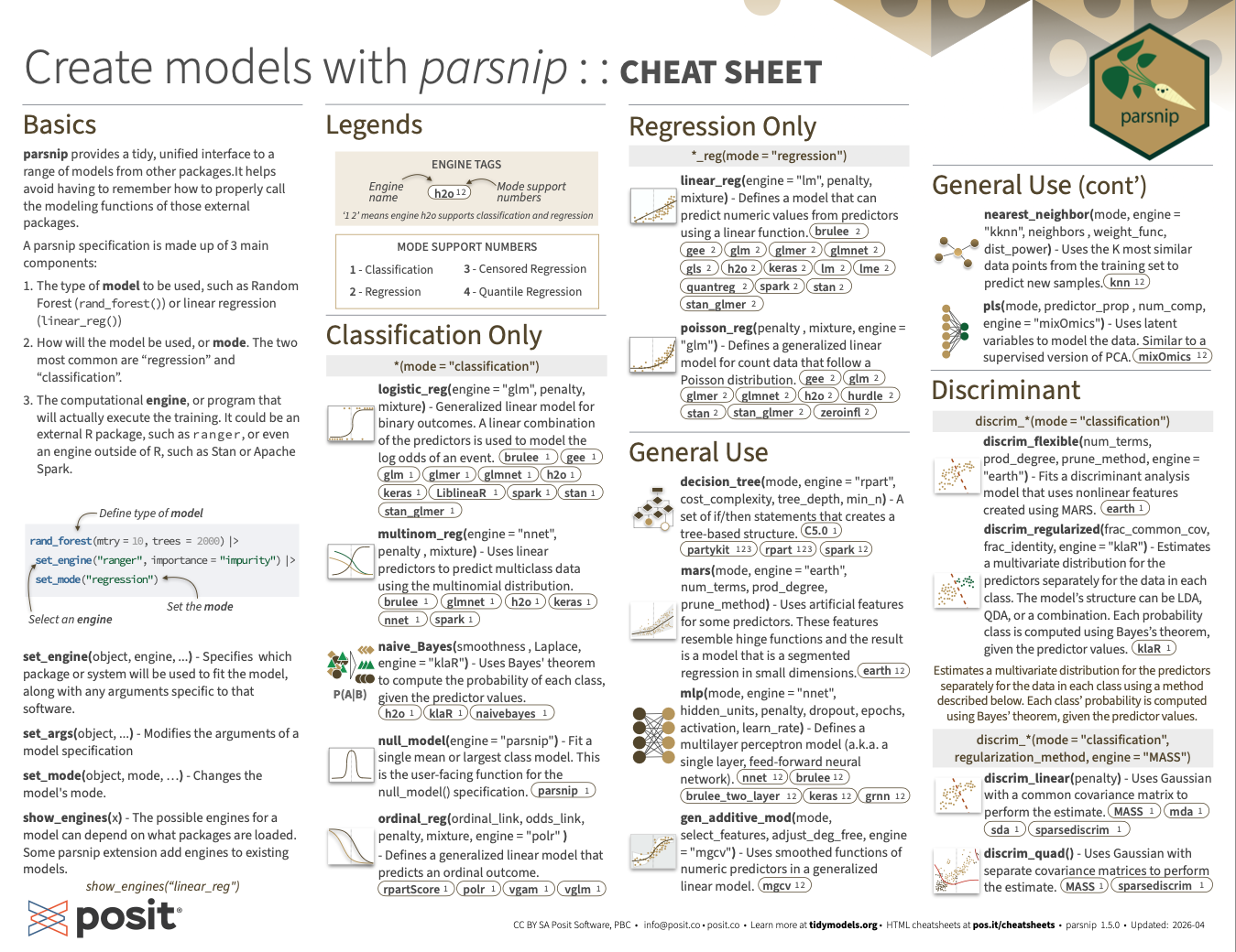
parsnip provides a tidy, unified interface to a range of models from other packages. It helps avoid having to remember how to properly call the modeling functions of those external packages.
A parsnip specification is made up of 3 main components:
The type of model to be used, such as Random Forest (
rand_forest()) or linear regression (linear_reg())How will the model be used, or mode. The two most common are “regression” and “classification”.
The computational engine, or program that will actually execute the training. It could be an external R package, such as ranger, or even an engine outside of R, such as Stan or Apache Spark.
library(tidymodels)

rand_forest(mtry = 10, trees = 2000) |> # Define type of model
  set_engine("ranger", importance = "impurity") |> # Select an engine
  set_mode("regression") # Set the mode
Random Forest Model Specification (regression)
Main Arguments:
mtry = 10
trees = 2000
Engine-Specific Arguments:
importance = impurity
Computational engine: ranger set_engine(object, engine, ...) - Specifies which package or system will be used to fit the model, along with any arguments specific to that software.
set_args(object, ...) - Modifies the arguments of a model specification
set_mode(object, mode, …) - Changes the model’s mode.
show_engines(x) - The possible engines for a model can depend on what packages are loaded. Some parsnip extension add engines to existing models.
show_engines("linear_reg")# A tibble: 8 × 2
engine mode
<chr> <chr>
1 lm regression
2 glm regression
3 glmnet regression
4 stan regression
5 spark regression
6 keras regression
7 brulee regression
8 quantreg quantile regressionLegends
Mode Support Numbers
- 1 - Classification
- 2 - Regression
- 3 - Censored Regression
- 4 - Quantile Regression
Classification Only
logistic_reg(mode = "classification", engine = "glm", penalty, mixture)- Generalized linear model for binary outcomes. A linear combination of the predictors is used to model the log odds of an event.brulee 1 gee 1 glm 1 glmer 1 glmnet 1 h2o 1 keras 1 LiblineaR 1 spark 1 stan 1 stan_glmer 1
multinom_reg(mode = "classification", engine = "nnet", penalty, mixture)- Uses linear predictors to predict multiclass data using the multinomial distribution.brulee 1 glmnet 1 h2o 1 keras 1 nnet 1 spark 1
naive_Bayes(mode = "classification", smoothness, Laplace, engine = "klaR")- Uses Bayes’ theorem to compute the probability of each class, given the predictor values.h2o 1 klaR 1 naivebayes 1
null_model(mode = "classification", engine = "parsnip")- Fit a single mean or largest class model. This is the user-facing function for the null_model() specification.parsnip 1
ordinal_reg(mode = "classification", ordinal_link, odds_link, penalty, mixture, engine = "polr")- Defines a generalized linear model that predicts an ordinal outcome.rpartScore 1 polr 1 vgam 1 vglm 1
Regression Only
linear_reg(mode = "regression", engine = "lm", penalty, mixture)- Defines a model that can predict numeric values from predictors using a linear function.brulee 2 gee 2 glm 2 glmer 2 glmnet 2 gls 2 h2o 2 keras 2 lm 2 lme 2 quantreg 2 spark 2 stan 2 stan_glmer 2
poisson_reg(mode = "regression", penalty, mixture, engine = "glm")- Defines a generalized linear model for count data that follow a Poisson distribution.gee 2 glm 2 glmer 2 glmnet 2 h2o 2 hurdle 2 stan 2 stan_glmer 2 zeroinfl 2
General Use
decision_tree(mode, engine = "rpart", cost_complexity, tree_depth, min_n)- A set of if/then statements creates a tree-based structure.partykit 123 rpart 123 spark 12 C5.0 1
mars(mode, engine = "earth", num_terms, prod_degree, prune_method)- Uses artificial features for some predictors. These features resemble hinge functions and the result is a model that is a segmented regression in small dimensions.earth 12
mlp(mode, engine = "nnet", hidden_units, penalty, dropout, epochs, activation, learn_rate)- Defines a multilayer perceptron model (a.k.a. a single layer, feed-forward neural network).nnet 12 brulee 12 brulee_two_layer 12 keras 12 grnn 12
gen_additive_mod(mode, select_features, adjust_deg_free, engine = "mgcv")- Uses smoothed functions of numeric predictors in a generalized linear model.mgcv 12
nearest_neighbor(mode, engine = "kknn", neighbors, weight_func, dist_power)- Uses the K most similar data points from the training set to predict new samples.knn 12
pls(mode, predictor_prop, num_comp, engine = "mixOmics")- Uses latent variables to model the data. Similar to a supervised version of PCA.mixOmics 12
Discriminant
discrim_flexible(mode = "classification", num_terms, prod_degree, prune_method, engine = "earth")- Fits a discriminant analysis model that uses nonlinear features created using MARS.earth 1
discrim_regularized(mode = "classification", frac_common_cov, frac_identity, engine = "klaR")- Estimates a multivariate distribution for the predictors separately for the data in each class. The model’s structure can be LDA, QDA, or a combination. Each probability class is computed using Bayes’s theorem, given the predictor values.klaR 1
Estimates a multivariate distribution for the predictors separately for the data in each class using a method described below. Each class’ probability is computed using Bayes’ theorem, given the predictor values.
discrim_linear(mode = "classification", regularization_method, engine = "MASS", penalty)- Uses Gaussian with a common covariance matrix to perform the estimate.MASS 1 mda 1 sda 1 sparsediscrim 1
discrim_quad(mode = "classification", regularization_method, engine = "MASS")- Uses Gaussian with separate covariance matrices to perform the estimate.MASS 1 sparsediscrim 1
Support Vector Machine
Classification: Maximizes the width of the margin between classes using a method described below.
Regression: Optimizes a robust loss function only affected by very large model residuals and uses an additional method described below.
svm_linear(mode, cost, engine = "LiblineaR", margin)- Classification: A linear class boundary. Regression: Uses a linear fit.kernlab 12 LiblineaR 12
svm_poly(mode, cost, engine = "kernlab", degree, scale_factor)- Classification: A polynomial class boundary. Regression: Uses polynomial functions of the predictors.kernlab 12
svm_rbf(mode, cost, engine = "kernlab", rbf_sigma)- Classification: A nonlinear class boundary. Regression: Uses nonlinear functions of the predictors.kernlab 12
Feature Rules
rule_fit(mode, mtry, trees, min_n, tree_depth, learn_rate, loss_reduction, sample_size, stop_iter, penalty, engine = "xrf")- Derives simple feature rules from a tree ensemble and uses them as features in a regularized model.xrf 12 h2o 1
C5_rules(mode = "classification", trees, min_n, engine = "C5.0")- Derives feature rules from a tree for prediction. A single tree or boosted ensemble can be used.C5.0 1
cubist_rules(mode = "regression", committees, neighbors, max_rules, engine = "Cubist")- Derives simple feature rules from a tree ensemble and creates regression models within each rule.Cubist 2
Ensemble
“E Pluribus Unum”
bag_mars(mode, num_terms, prod_degree, prune_method, engine = "earth")- Ensemble of generalized linear models that use artificial features for some predictors. These features resemble hinge functions and the result is a model that is a segmented regression in small dimensions.earth 12
bag_mlp(mode, hidden_units, penalty, epochs, engine = "nnet")- An ensemble of single layer, feed-forward neural networks.nnet 12
bag_tree(mode, cost_complexity = 0, tree_depth, min_n = 2, class_cost, engine = "rpart")- Ensemble of decision trees.C5.0 1 rpart 123
bart(mode, engine = "dbarts", trees, prior_terminal_node_coef, prior_terminal_node_expo, prior_outcome_range)- Tree ensemble model that uses Bayesian analysis to assemble the ensemble.bart 12
boost_tree(mode, engine = "xgboost", mtry, trees, min_n, tree_depth, learn_rate, loss_reduction, sample_size, stop_iter)- Creates a series of decision trees forming an ensemble. Each tree depends on the results of previous trees. All trees in the ensemble are combined to produce a final prediction.C5.0 1 catboost 12 h2o 12 lightgbm 12 mboost 3 spark 12 xgboost 124
rand_forest(mode, engine = "ranger", mtry, trees, min_n)- Creates a large number of decision trees, each independent of the others. The final prediction uses all predictions from the individual trees and combines them.aorsf 123 grf 124 h2o 12 partykit 123 randomForest 12 ranger 12 spark 12
Survival
proportional_hazards(mode = "censored regression", engine = "survival", penalty, mixture)- Defines a model for the hazard function as a multiplicative function of covariates times a baseline hazard.glmnet 3 survival 3
survival_reg(mode = "censored regression", engine = "survival", dist)- Defines a parametric survival model.flexsurv 3 flexsurvspline 3 survival 3
Operations
library(tidymodels)

lm_spec <- linear_reg() |>
  set_engine("lm")

lm_spec
Linear Regression Model Specification (regression)
Computational engine: lm Methods
fit(object, ...)- Estimates parameters for a given model from a set of data.lm_fit <- fit(lm_spec, mpg ~ ., data = mtcars) lm_fitparsnip model object Call: stats::lm(formula = mpg ~ ., data = data) Coefficients: (Intercept) cyl disp hp drat wt 12.30337 -0.11144 0.01334 -0.02148 0.78711 -3.71530 qsec vs am gear carb 0.82104 0.31776 2.52023 0.65541 -0.19942predict(object, ...)predict(lm_fit, mtcars)# A tibble: 32 × 1 .pred <dbl> 1 22.6 2 22.1 3 26.3 4 21.2 5 17.7 6 20.4 7 14.4 8 22.5 9 24.4 10 18.7 # ℹ 22 more rowsautoplot(object, ...)- Uses ggplot2 to draw a particular plot for an object of a particular classupdate(object, ...)- Updates and (by default) re-fit a model. It does this by extracting the call stored in the object, updating the call and evaluating that call.
Tidiers
augment(x, ...)- Augment data with model resultsaugment(lm_fit, mtcars)# A tibble: 32 × 13 .pred .resid mpg cyl disp hp drat wt qsec vs am gear <dbl> <dbl> <dbl> <dbl> <dbl> <dbl> <dbl> <dbl> <dbl> <dbl> <dbl> <dbl> 1 22.6 -1.60 21 6 160 110 3.9 2.62 16.5 0 1 4 2 22.1 -1.11 21 6 160 110 3.9 2.88 17.0 0 1 4 3 26.3 -3.45 22.8 4 108 93 3.85 2.32 18.6 1 1 4 4 21.2 0.163 21.4 6 258 110 3.08 3.22 19.4 1 0 3 5 17.7 1.01 18.7 8 360 175 3.15 3.44 17.0 0 0 3 6 20.4 -2.28 18.1 6 225 105 2.76 3.46 20.2 1 0 3 7 14.4 -0.0863 14.3 8 360 245 3.21 3.57 15.8 0 0 3 8 22.5 1.90 24.4 4 147. 62 3.69 3.19 20 1 0 4 9 24.4 -1.62 22.8 4 141. 95 3.92 3.15 22.9 1 0 4 10 18.7 0.501 19.2 6 168. 123 3.92 3.44 18.3 1 0 4 # ℹ 22 more rows # ℹ 1 more variable: carb <dbl>glance(x, ...)- Construct a single row summary “glance” of a model fitglance(lm_fit)# A tibble: 1 × 12 r.squared adj.r.squared sigma statistic p.value df logLik AIC BIC <dbl> <dbl> <dbl> <dbl> <dbl> <dbl> <dbl> <dbl> <dbl> 1 0.869 0.807 2.65 13.9 0.000000379 10 -69.9 164. 181. # ℹ 3 more variables: deviance <dbl>, df.residual <int>, nobs <int>tidy(x, ...)- Turn an object into a tidy tibbletidy(lm_fit)# A tibble: 11 × 5 term estimate std.error statistic p.value <chr> <dbl> <dbl> <dbl> <dbl> 1 (Intercept) 12.3 18.7 0.657 0.518 2 cyl -0.111 1.05 -0.107 0.916 3 disp 0.0133 0.0179 0.747 0.463 4 hp -0.0215 0.0218 -0.987 0.335 5 drat 0.787 1.64 0.481 0.635 6 wt -3.72 1.89 -1.96 0.0633 7 qsec 0.821 0.731 1.12 0.274 8 vs 0.318 2.10 0.151 0.881 9 am 2.52 2.06 1.23 0.234 10 gear 0.655 1.49 0.439 0.665 11 carb -0.199 0.829 -0.241 0.812
General
repair_call(x, data)- When the user passes a formula to fit() and the underlying model function uses a formula, the call object produced by fit() may not be usable by other functions.control_parsnip(verbosity = 1L, catch = FALSE)- Pass options to the fit.model_spec() function to control its output and computations.control_parsnip(verbosity = 2)parsnip control object - verbose level 2show_engines(x)- The possible engines for a model can depend on what packages are loaded. Some parsnip extension add engines to existing models.show_engines("linear_reg")# A tibble: 8 × 2 engine mode <chr> <chr> 1 lm regression 2 glm regression 3 glmnet regression 4 stan regression 5 spark regression 6 keras regression 7 brulee regression 8 quantreg quantile regressiontranslate(x, ...)- Translates a model specification into a code object that is specific to a particular engine (e.g. R package). It translates generic parameters to their counterparts.translate(lm_spec)Linear Regression Model Specification (regression) Computational engine: lm Model fit template: stats::lm(formula = missing_arg(), data = missing_arg(), weights = missing_arg())multi_predict(object, ...)- For some models, predictions can be made on sub-models in the model object.
Extract
extract_spec_parsnip(x, ...)- Returns a parsnip model specification.extract_spec_parsnip(lm_fit)Linear Regression Model Specification (regression) Computational engine: lm Model fit template: stats::lm(formula = missing_arg(), data = missing_arg(), weights = missing_arg())extract_fit_engine(x, ...)- Returns the engine specific fit embedded within a parsnip model fit. For example, when using linear_reg() with the “lm” engine, this returns the underlying lm object.extract_fit_engine(lm_fit)Call: stats::lm(formula = mpg ~ ., data = data) Coefficients: (Intercept) cyl disp hp drat wt 12.30337 -0.11144 0.01334 -0.02148 0.78711 -3.71530 qsec vs am gear carb 0.82104 0.31776 2.52023 0.65541 -0.19942extract_parameter_dials(x, parameter, ...)- Returns a single dials parameter object.extract_parameter_set_dials(x, ...)- Returns a set of dials parameter objects.extract_fit_time(x, summarize = TRUE, ...)- returns a tibble with fit times. The fit times correspond to the time for the parsnip engine to fit and do not include other portions of the elapsed time in fit.model_spec().