Frequently asked questions
- Why do some function calls not show in the profiler?
- How do I share a profvis visualization?
- What does
<Anonymous>mean? - What does
cmpfunmean? - How do I get code from an R package to show in the code panel?
- Can I profile code without calling
profvis()? - Why does the flame graph hide some function calls for Shiny apps?
- Can I profile just part of a Shiny application?
- Can I profile a Shiny application running on a remote server?
- Why does
Sys.sleep()not show up in profiler data? - Why is the call stack reversed for some of my code?
- Why does profvis tell me the the wrong line is taking time?
- How do I interpret memory profiling information?
- How do I split the panes vertically instead of horizontally?
- How do I get source code to show with
Rscript? - What are some other resources for profiling R code?
Why do some function calls not show in the profiler?
As noted earlier, some of R’s built-in functions don’t show in the profvis flame graph. These include functions like <-, [, and $. Although these functions can occupy a lot of time, they don’t show on the call stack. (In one of the examples above, $ does show on the call stack, but this is because it was dispatched to $.data.frame, as opposed to R’s internal C code, which is used for indexing into lists.)
In some cases the side-effects of these functions can be seen in the flamegraph. As we saw in the example above, using these functions in a loop led to many memory allocations, which led to garbage collections, or <GC> blocks in the flame graph.
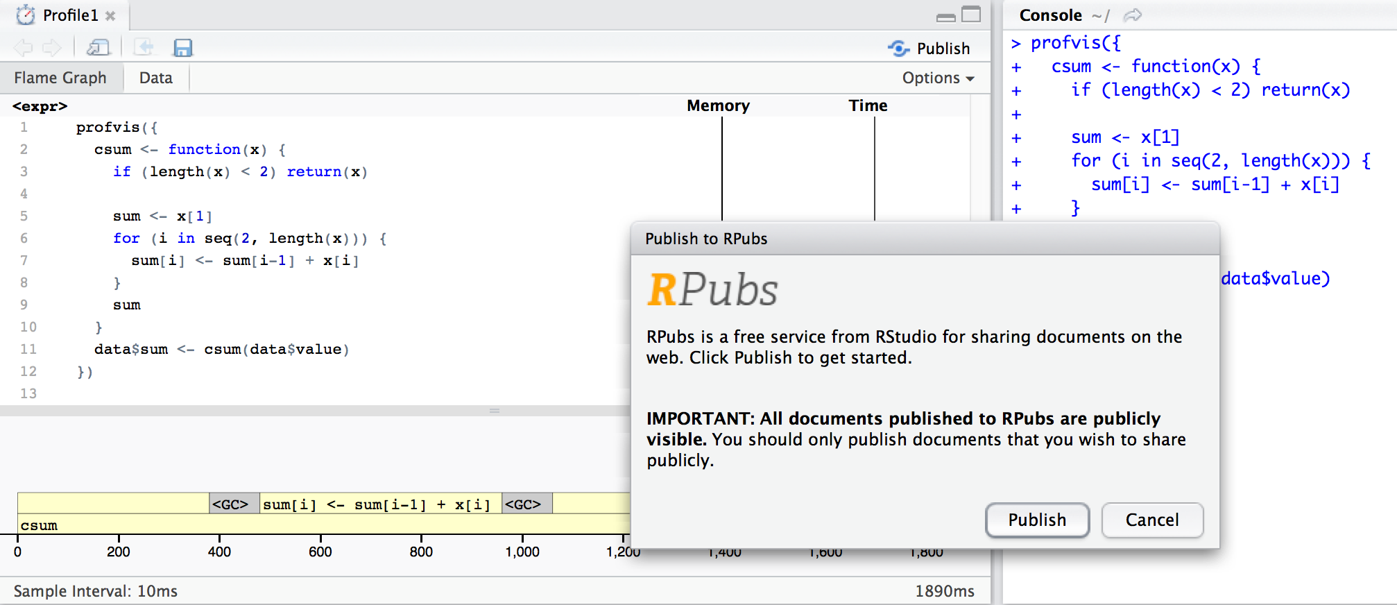
How do I share a profvis visualization?
Right now the easiest way to do this is to run profvis in RStudio, and publish to RPubs.
Once the profile shows up in the RStudio IDE, click on the Publish button to send it to RPubs. You can see an example here. If you don’t already have an account on RPubs, you’ll need to set one up.
You can also click on the save (disk) icon. This will save the profvis visualization to an .Rprofvis file. This file can be opened by RStudio, or if you rename it to have an .html extension, it can be opened in a web browser.
Publishing to RPubs
Another way to publish a profvis visualization is to save the HTML output file using htmlwidgets::saveWidget, and put that on any web hosting service:
p <- profvis({
  # Interesting code here
})

htmlwidgets::saveWidget(p, "profile.html")
It’s also possible to put a profvis visualization in a knitr document. At this time, some CSS workarounds are needed needed for them to display properly. You can look at the source of this website to see the workarounds.
What does <Anonymous> mean?
It’s not uncommon for R code to contain anonymous functions – that is, functions that aren’t named. These show up as <Anonymous> in the profiling data collected from Rprof.
In the code below there is a function, make_adder, that returns a function. We’ll invoke the returned function in two ways.
First, we’ll run make_adder(1)(10). The call make_adder(1) returns a function, which is invoked immediately (without being saved in a variable), and shows up as <Anonymous> in the flame graph.
Next, we’ll call make_adder(2) but this time, we’ll save the result in a variable, adder2. Then we’ll call adder2(10). When we do it this way, the profiler records that the function label is adder2.
profvis({
  make_adder <- function(n) {
    function(x) {
      pause(0.25) # Wait for a moment so that this shows in the profiler
      x + n
    }
  }

  # Called with no intermediate variable, it shows as "<Anonymous>"
  make_adder(1)(10)

  # With the function saved in a variable, it shows as "adder2"
  adder2 <- make_adder(2)
  adder2(10)
})
Similarly, in versions of R before 3.3.0, functions that are accessed with :: or $ will also appear as <Anonymous>. The form package::function() is a common way to explicitly use a namespace to find a function. The form x$fun() is a common way to call functions that are contained in a list, environment, reference class, or R6 object. As of R 3.3.0, these will display as package::function, or x$fun.
Those are equivalent to `::`(package, function) and `$`(x, "fun"), respectively. These calls return anonymous functions, and so R’s internal profiling code labels these as <Anonymous>. If you want labels in the profiler to have a different label, you can assign the value to a temporary variable (like adder2 above), and then invoke that.
Finally, if a function is passed to lapply, it will be show up as FUN in the flame graph. If we inspect the source code for lapply, it’s clear why: when a function is passed to lapply, the name used for the function inside of lapply is FUN.
lapply
#> function (X, FUN, ...)
#> {
#>     FUN <- match.fun(FUN)
#>     if (!is.vector(X) || is.object(X))
#>         X <- as.list(X)
#>     .Internal(lapply(X, FUN))
#> }
#> <bytecode: 0x7fa19d09efc0>
#> <environment: namespace:base>
What does cmpfun mean?
The first time we run profvis on a function in a clean 3.4.0 or greater R session, we’ll see compiler:::tryCmpfun. For example,
profvis({
  data <- data.frame(value = runif(5e4))

  csum <- function(x) {
    if (length(x) < 2) return(x)

    sum <- x[1]
    for (i in seq(2, length(x))) {
      sum[i] <- sum[i-1] + x[i]
    }
    sum
  }
  data$sum <- csum(data$value)
})
As of R 3.4.0, R attempts to compile functions when they are first ran to byte code. On subsequent function calls, instead of reinterpreting the body of the function, R executes the saved and compiled byte code. Typically, this results in faster execution times on later function calls. For example, let’s profile csum a second time in the same R session:
Now the flame graph shows that the function is no longer being compiled. And after compiling, csum is about 40 ms faster.
How do I get code from an R package to show in the code panel?
In typical use, only code written by the user is shown in the code panel. (This is code for which source references are available.) Yellow blocks in the flame graph have corresponding lines of code in the code panel, and when moused over, the line of code will be highlighted. White blocks in the flame graph don’t have corresponding lines in the code panel. In most cases, the calls represented by the white blocks are to functions that are in base R and other packages.
Profvis can also show code that’s inside an R package. To do this, source refs for the package code must be available. There are two general ways to do this: you can install the package with source refs, or you can use devtools::load_all() to load a package from sources on disk.
Installing with source refs
There are many ways to install a package with source refs. Here are some examples of installing ggplot2:
From CRAN:
## First, restart R ##
install.packages("ggplot2", type="source", INSTALL_opts="--with-keep.source")
From an RStudio package project on local disk: Go to Build -> Configure Build Tools -> Build Tools -> Build and Reload – R CMD INSTALL additional options, and add
--with-keep.source. Then run Build -> Build and Reload.From sources on disk with devtools:
## First, restart R ##
# Assuming sources are in a subdirectory ggplot2/
devtools::install("ggplot2", keep_source = TRUE)
From sources on disk using the command line:
R CMD INSTALL --with-keep.source ggplot2/From sources on Github:
## First, restart R ##
remotes::install_github("hadley/ggplot2", INSTALL_opts="--with-keep.source")
Loading packages with source refs (without installing)
Instead of installing an in-development package, you can simply load it from source using devtools.
# Assuming sources are in a subdirectory ggplot2/
devtools::load_all("ggplot2")
Once a package is loaded or installed with source refs, profvis visualizations will display source code for that package. For example, the visualization below has yellow blocks for both user code and for code in ggplot2, and it contains ggplot2 code in the code panel:
library(ggplot2)
profvis({
  g <- ggplot(diamonds, aes(carat, price)) + geom_point(size = 1, alpha = 0.2)
  print(g)
})
Can I profile code without calling profvis()?
Yes. There are two ways to do it.
If you are in RStudio, you can select Profile->Start Profiling, run your code, and then Profile->Stop Profiling. When you stop the profiling, the profvis viewer will come up.
Another way is to start and stop the R profiler manually, then have profvis read in the recorded profiling data. To profile your code, run:
# Start profiler
Rprof("data.Rprof", interval = 0.01, line.profiling = TRUE,
      gc.profiling = TRUE, memory.profiling = TRUE)

## Run your code here

# Stop profiler
Rprof(NULL)
Then you can load the data into profvis:
profvis(prof_input = "data.Rprof")This technique can also be used to profile just one section of your code.
Why does the flame graph hide some function calls for Shiny apps?
When profiling Shiny applications, the profvis flame graph will hide many function calls by default. They’re hidden because they aren’t particularly informative for optimizing code, and they add visual complexity. This feature requires Shiny 0.13.0 or greater.
If you want to see these hidden blocks, uncheck Options -> Hide internal function calls:
library(shiny)
profvis({
  # After this app has started, interact with it a bit, then quit
  runExample("06_tabsets", display.mode = "normal")
})
To make the hiding work, Shiny has special functions called ..stacktraceon.. and ..stacktraceoff... Profvis goes up the stack, and when it sees a ..stacktraceoff.., it will hide all function calls until it sees a corresponding ..stacktraceon... If there are nukltiple ..stacktraceoff.. calls in the stack, it requires an equal number of ..stacktraceon.. calls before it starts displaying function calls again.
Can I profile just part of a Shiny application?
Sometimes it it useful to profile just part of a Shiny application, instead of the whole thing from start to finish.
If you are in RStudio, you can start your application, then select Profile->Start Profiling, interact with your application, and then select Profile->Stop Profiling. When you stop the profiling, the profvis viewer will come up.
Profivs also provides a Shiny Module to initiate the profiling, and provides a UI to start, stop, view, and download profvis sessions. This is done with profvis::profvis_server and profvis::profvis_ui.
For example, here’s a small app that uses the module:
library(shiny)
library(ggplot2)
library(profvis)
shinyApp(
  fluidPage(
    plotOutput("plot"),
    actionButton("new", "New plot"),
    profvis_ui("profiler")
  ),
  function(input, output, session) {
    callModule(profvis_server, "profiler")

    output$plot <- renderPlot({
      input$new
      ggplot(diamonds, aes(carat, price)) + geom_point()
    })
  }
)
In the server function, callModule(profvis_server, "profiler") sets up the profvis session, and in the UI profvis_ui("profiler") sets up a basic interface to start, stop, view, and download profvis sessions.
You can create your own profvis_server and profvis_ui functions by calling Rprof() to start and stop profiling (as described in this answer), and trigger it with an actionButton. For example, you could put this in your UI:
radioButtons("profile", "Profiling", c("off", "on"))And put this in your server function:
  observe({
    if (identical(input$profile, "off")) {
      Rprof(NULL)
    } else if (identical(input$profile, "on")){
      Rprof(strftime(Sys.time(), "%Y-%m-%d-%H-%M-%S.Rprof"),
            interval = 0.01, line.profiling = TRUE,
            gc.profiling = TRUE, memory.profiling = TRUE)
    }
  })
It will add radio buttons to turn profiling on and off. Turn it on, then interact with your app, then turn it off. There will be a file with a name corresponding to the start time. You can view the profiler output with profvis, with something like this:
profvis(prof_input = "2018-08-07-12-22-35.Rprof")Can I profile a Shiny application running on a remote server?
Yes. One option is to include the Profvis Shiny Module desribed in the previous question.
You can also set it up manually. The main idea is to start and stop profiling (as described in this answer). At the top of your app.R or server.R, you can add the following:
Rprof(strftime(Sys.time(), "%Y-%m-%d-%H-%M-%S.Rprof"),
      interval = 0.01, line.profiling = TRUE,
      gc.profiling = TRUE, memory.profiling = TRUE)

onStop(function() {
  Rprof(NULL)
})
This will start profiling when the app starts, and stop when it exits.
Why does Sys.sleep() not show up in profiler data?
The R profiler doesn’t provide any data when R makes a system call. If, for example, you call Sys.sleep(5), the R process will pause for 5 seconds, but you probably won’t see any instances of Sys.sleep in the profvis visualization – it won’t even take any horizontal space. For these examples, we’ve used the pause function instead, which is part of the profvis package. It’s similar to Sys.sleep, except that it does show up in the profiling data. For example:
profvis({
  # Does not show in the flame graph
  Sys.sleep(0.25)

  # Does show in the flame graph
  pause(0.25)
})
Calls to external programs and libraries also may not show up in the profiling data. If you call functions from a package to fetch data from external sources, keep in mind that time spent in those functions may not show in the profiler.
Why is the call stack reversed for some of my code?
One of the unusual features of R as a programming language is that it has lazy evaluation of function arguments. If you pass an expression to a function, that expression won’t be evaluated until it’s actually used somewhere in that function.
The result of this is that sometimes the stack can look like it’s in the wrong order. In this example below, we call times_10 and times_10_lazy. They both call times_5() and times_2(), but the “regular” version uses an intermediate variable y, while the lazy version nests the calls, with times_2(times_5(x)).
profvis({
  times_5 <- function(x) {
    pause(0.5)
    x * 5
  }

  times_2 <- function(x) {
    pause(0.2)
    x * 2
  }

  times_10 <- function(x) {
    y <- times_5(x)
    times_2(y)
  }

  times_10_lazy <- function(x) {
    times_2(times_5(x))
  }

  times_10(10)
  times_10_lazy(10)
})
In most programming languages, the flame graph would look the same for both: the times_10 (or times_10_lazy) block would be on the bottom, with times_5 and times_2 side-by-side on the next level up on the stack.
With lazy evaluation, when the times_10_lazy function calls times_2(times_5(x)), the times_2 function receives a promise with the unevaluated expression times_5(x), and evaluates it only when it reaches line 9, x * 2 (the expression gets evaluated in the correct context, so there’s no naming collision of the x variable).
It’s not only the call stack that has a surprising order with times_10_lazy – the temporal order the simulated work we’re doing in the function (represented by the pause blocks) is different. The times_2 and times_5 functions pause for 0.2 and 0.5 seconds, respectively. Those pauses occur in opposite order in times_10 and times_10_lazy.
Keep in mind that lazy evaluation may result in counterintuitive results in the flame graph. If you want to avoid some of the possible confusion from lazy evaluation, you can use intermediate variables to force the evaluation of arguments at specific locations in your code, as we did in times_10.
Why does profvis tell me the the wrong line is taking time?
In some cases, multi-line expressions will report that the first line of the expression is the one that takes all the time. In the example below, there are two for loops: one with curly braces, and one without. In the loop with curly braces, it reports that line 3, containing the pause is the one that takes all the time. In the loop without curly braces, it reports that line 6, containing for, is the one that takes all the time, even though the time is really spent on line 7, with the pause.
profvis({
  for (i in 1:3) {
    pause(0.1)
  }

  for (i in 1:3)
    pause(0.1)

})
For code that contains multi-line expressions like these, using curly braces will allow the profiler to identify the correct line where code is running.
How do I interpret memory profiling information?
The memory profiling information can be somewhat tricky to interpret, for two reasons. The first reason is that, compared to call stack information, memory usage information is collected with different temporal characteristics: call stack information is recorded instantaneously at each sample, while memory information is recorded between each sample.
The second reason that is that memory deallocations happen somewhat randomly, and may happen long after the point where the memory was no longer needed. The deallocations occur in garbage collection (<GC>) events.
For these reasons, it might look like a particular line of code (or function call in the flame graph) is responsible for memory allocation or deallocation, when in reality the memory use is due to a previous line of code.
If a section of code results in a large amount of allocation and deallocation, it means that it’s “churning” through memory and using a large amonut of temporary memory storage. This can be seen in Example 1 above. In these cases, it may be possible to optimize the code so that it doesn’t use as much temporary memory.
If a section of code results in a large amount of allocation but does not have a large amount of deallocation, then it means the memory is not being released. This could be because the code genuinely requires that extra memory, but it could also be a sign of a memory leak.
How do I split the panes vertically instead of horizontally?
The profvis examples in this document have a vertical split, but by default, profvis visualizations have a horizontal split. To switch directions, you can check or uncheck Options -> Split horizontally.
To change the split direction when the visualization opens, use split="v":
profvis({
  # Code here
}, split = "v")


# Also possible to control the split when calling print()
p <- profvis({
  # Code here
})
print(p, split = "v")
How do I get source code to show with Rscript?
If you run profvis from a script, the source code won’t show in the source panel. This is because source refs are not recorded by default when R is run non-interactively. To make it work, use options(keep.source=TRUE). For example:
Rscript -e "options(keep.source=TRUE); p <- profvis::profvis({ profvis::pause(0.2) }); htmlwidgets::saveWidget(p, 'test.html')"What are some other resources for profiling R code?
Base R comes with the Rprof function (it’s what profvis calls to collect profiling data) as well as the summaryRprof function for getting a human-readable summary of the profiling data collected by Rprof.
Luke Tierney and Riad Jarjour have authored the proftools package, which provides many more tools for summarizing profiling data, including hot paths, call summaries, and call graphs. Proftools can also be used to generate a number of visualizations, including call graphs, flame graphs, and callee tree maps.