9 Intro to dashboards

9.1 Basic structure

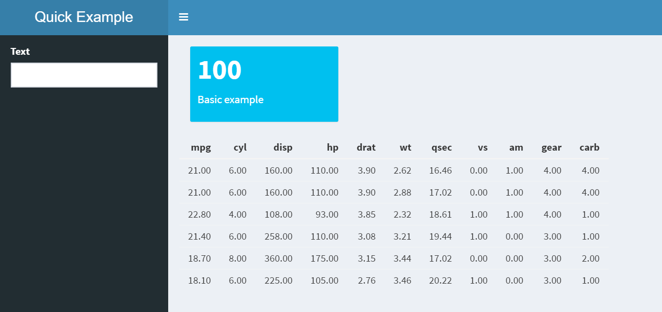
Preview a simple shinydashboard

1. Create and preview a simple shinydashboard

ui <- dashboardPage(
  dashboardHeader(title = "Quick Example"),
  dashboardSidebar(selectInput("select", "Selection", c("one", "two"))),
  dashboardBody(
    valueBoxOutput("total"),
    dataTableOutput("monthly")
  )
)

server <- function(input, output, session) {
  output$total <- renderValueBox(valueBox(100, subtitle = "Flights"))
  output$monthly <- renderDataTable(datatable(mtcars))
}

shinyApp(ui, server)

9.2 Dropdown data

Review a technique to populate a dropdown

1. Use purrr to create a list with the correct structure for the shiny drop down

airline_list <- carriers %>%  
  select(carrier, carriername) %>%   # In case more fields are added
  collect()  %>%                     # All would be collected anyway
  split(.$carriername) %>%           # Create a list item for each name
  map(~.$carrier)                    # Add the carrier code to each item

head(airline_list)

## $`AirTran Airways Corporation`
## [1] "FL"
## 
## $`Alaska Airlines Inc.`
## [1] "AS"
## 
## $`Aloha Airlines Inc.`
## [1] "AQ"
## 
## $`American Airlines Inc.`
## [1] "AA"
## 
## $`American Eagle Airlines Inc.`
## [1] "MQ"
## 
## $`Atlantic Southeast Airlines`
## [1] "EV"

2. In the app code, replace c("one", "two", "three") with airline_list

# Goes from this:
dashboardSidebar(selectInput("select", "Selection", c("one", "two"))),
# To this:
dashboardSidebar(selectInput("select", "Selection", airline_list)),

3. Re-run the app

9.3 Update dashboard items

Create base query for the dashboard using dplyr and pass the results to the dashboard

1. Save the base “query” to a variable. It will contain a carrier selection. To transition into shiny programming easier, the variable will be a function.

base_dashboard <- function(){
  flights %>%
    filter(uniquecarrier == "DL")
  }

head(base_dashboard())

## # Source:   lazy query [?? x 31]
## # Database: postgres [rstudio_dev@localhost:/postgres]
##   flightid  year month dayofmonth dayofweek deptime crsdeptime arrtime
##      <int> <dbl> <dbl>      <dbl>     <dbl>   <dbl>      <dbl>   <dbl>
## 1   900594  2008     2         22         5      NA       1555      NA
## 2   900595  2008     2         22         5      NA        755      NA
## 3   900639  2008     2         22         5      NA        930      NA
## 4   899610  2008     2         22         5     753        800      NA
## 5   900640  2008     2         22         5      NA       1030      NA
## 6   900641  2008     2         22         5      NA       1030      NA
## # … with 23 more variables: crsarrtime <dbl>, uniquecarrier <chr>,
## #   flightnum <dbl>, tailnum <chr>, actualelapsedtime <dbl>,
## #   crselapsedtime <dbl>, airtime <dbl>, arrdelay <dbl>, depdelay <dbl>,
## #   origin <chr>, dest <chr>, distance <dbl>, taxiin <dbl>, taxiout <dbl>,
## #   cancelled <dbl>, cancellationcode <chr>, diverted <dbl>,
## #   carrierdelay <dbl>, weatherdelay <dbl>, nasdelay <dbl>,
## #   securitydelay <dbl>, lateaircraftdelay <dbl>, score <int>

3. Use the base query to figure the number of flights for that carrier

base_dashboard() %>%
  tally() %>% 
  pull()

## integer64
## [1] 451931

4. In the app, remove the 100 number and pipe the dplyr code into the valueBox() function

# Goes from this:
  output$total <- renderValueBox(valueBox(100, subtitle = "Flights"))
# To this:
  output$total <- renderValueBox(
    base_dashboard() %>%
      tally() %>% 
      pull() %>%
      valueBox(subtitle = "Flights"))

5. Create a table with the month name and the number of flights for that month

base_dashboard() %>%
  group_by(month) %>%
  tally() %>%
  collect() %>%
  mutate(n = as.numeric(n)) %>%
  rename(flights = n) %>%
  arrange(month)

## # A tibble: 12 x 2
##    month flights
##    <dbl>   <dbl>
##  1     1   38256
##  2     2   36275
##  3     3   39829
##  4     4   37049
##  5     5   36349
##  6     6   37844
##  7     7   39335
##  8     8   38173
##  9     9   36304
## 10    10   38645
## 11    11   36939
## 12    12   36933

6. In the app, replace head(mtcars) with the piped code, and re-run the app

# Goes from this:
  output$monthly <- renderTable(head(mtcars))
# To this:
  output$monthly <- renderDataTable(datatable(
    base_dashboard() %>%
      group_by(month) %>%
      tally() %>%
      collect() %>%
      mutate(n = as.numeric(n)) %>%
      rename(flights = n) %>%
      arrange(month)))

9.4 Integrate the dropdown

Use shiny’s reactive() function to integrate the user input in one spot

1. In the original base_dashboard() code, replace function with reactive, and "DL" with input$select

# Goes from this
base_dashboard <- function(){
flights %>%
  filter(uniquecarrier == "DL")}
# To this
base_dashboard <- reactive({
  flights %>% 
    filter(uniquecarrier == input$select)})

2. Insert the new code right after the server <- function(input, output, session) line. The full code should now look like this:

ui <- dashboardPage(
  dashboardHeader(title = "Quick Example"),
  dashboardSidebar(selectInput("select", "Selection", airline_list)),
  dashboardBody(
    valueBoxOutput("total"),
    dataTableOutput("monthly")
  )
)

server <- function(input, output, session) {
  base_dashboard <- reactive({
    flights %>%
      filter(uniquecarrier == input$select)
  })
  output$total <- renderValueBox(
    base_dashboard() %>%
      tally() %>%
      pull() %>%
      valueBox(subtitle = "Flights")
  )
  output$monthly <- renderDataTable(datatable(
    base_dashboard() %>%
      group_by(month) %>%
      tally() %>%
      collect() %>%
      mutate(n = as.numeric(n)) %>%
      rename(flights = n) %>%
      arrange(month)
  ))
}
shinyApp(ui, server)

9. Re-run the app

10. Disconnect form database

dbDisconnect(con)

#Dashboard drill-down

9.5 Add a tabset to the dashboard

Prepare the ui to accept new tabs based on the user’s input

1. Wrap the “output” functions in the ui with a tabPanel()

# Goes from this
valueBoxOutput("total"),
dataTableOutput("monthly")

# To this
tabPanel(
  valueBoxOutput("total"),
  dataTableOutput("monthly")
  )

2. Set the panel’s title and value. The new code should look like this

tabPanel(
  title = "Dashboard", 
  value = "page1", 
  valueBoxOutput("total"),
  dataTableOutput("monthly")
  )

3. Wrap that code inside a tabsetPanel(), set the id to tabs

tabsetPanel(
  id = "tabs",
  tabPanel(
    title = "Dashboard",
    value = "page1",
    valueBoxOutput("total"),
    dataTableOutput("monthly")
  )
)

4. Re-run the app

9.6 Add interactivity

Add an click-event that creates a new tab

1. Set the selection and rownames in the current datatable() function

output$monthly <- renderDataTable(datatable({
  base_dashboard() %>%
    group_by(month) %>%
    tally() %>%
    collect() %>%
    mutate(n = as.numeric(n)) %>%
    rename(flights = n) %>%
    arrange(month)}, 
  list( target = "cell"),    # New code
  rownames = FALSE))         # New code

2. Use observeEvent() and appendTab() to add the interactivity

observeEvent(input$monthly_cell_clicked, {
  appendTab(
    inputId = "tabs", # This is the tabsets panel's ID
    tabPanel(
      "test_new", # This will be the label of the new tab
      renderDataTable(mtcars, rownames = FALSE)
    )
  )
}) 

3. Re-run the app

4. Click on a row inside the datatable and then select the new tab called test_new to see the mtcars data

9.7 Add title to the new tab

Use the input’s info to create a custom label

1. Load the clicked cell’s info into a variable, and create a new lable by concatenating the cell’s month and the selected airline’s code

observeEvent(input$monthly_cell_clicked, {
  cell <- input$monthly_cell_clicked # New code

  if (!is.null(cell$value)) { # New code
    tab_title <- paste0(month.name[cell$value], "_", input$select)
    appendTab(
      inputId = "tabs",
      tabPanel(
        tab_title, # Changed code
        renderDataTable(mtcars, rownames = FALSE)
      )
    )
  }
})

2. Re-run the app, and click on one of the month’s to confirm that the new label works

3. Use updateTabsetPanel to switch the dashboard’s focus to the newly created tab. It goes after the tabPanel() code

updateTabsetPanel(session, "tabs", selected = tab_title)

9.8 pool pakcage

Improve connectivity using the pool package

1.Change dbConnect() to dbPool()

# Goes from this
con <- DBI::dbConnect(odbc::odbc(), "Postgres Dev")

# To this
con <- pool::dbPool(odbc::odbc(), dsn =  "Postgres Dev")

2. Add an onStop() step to close the pool connection

onStop(function() {
  poolClose(con)
})

#Share and Production

9.9 Publish dashboard

Use RStudio Connect to publish work internally in the enterprise

1. Open the dashboard app.R file

2. Click on File

3. Click on Publish

4. Connect Account click Next

5. Select RStudio Connect

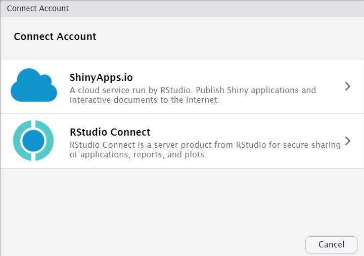
6. Copy and paste your RStudio Server URL and add :3939

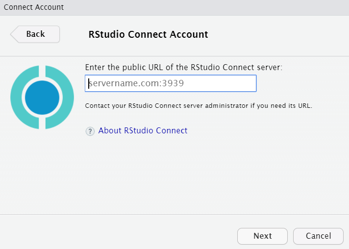
7. Enter your credentials

8. Complete the form

9. Click Proceed

10. Click on Connect

11. Click Publish

9.10 Schedule scoring

Use the tidypredict model to score and write back to the database

1. Create a new RMarkdown

2. Start the new RMarkdown by loading all the needed libraries, connecting to the DB and setting table_flights

3. Read the parsed model saved in exercise 5.6

my_pm <- yaml::read_yaml("my_model.yml")

4. Copy the code from exercise 5.5 step 4. Load the code into a variable called predictions. Change the model variable to parsedmodel

predictions <- table_flights %>%
  filter(month == 2,
         dayofmonth == 1) %>%
    mutate(
    season = case_when(
      month >= 3 & month <= 5  ~ "Spring",
      month >= 6 & month <= 8  ~ "Summmer",
      month >= 9 & month <= 11 ~ "Fall",
      month == 12 | month <= 2  ~ "Winter"
    )
  ) %>%
  select( season, depdelay) %>%
  tidypredict_to_column(parsedmodel) %>%
  remote_query()

5. Change the select() verb to include flightid, and rename to p_flightid

predictions <- table_flights %>%
  filter(month == 2,
         dayofmonth == 1) %>%
    mutate(
    season = case_when(
      month >= 3 & month <= 5  ~ "Spring",
      month >= 6 & month <= 8  ~ "Summmer",
      month >= 9 & month <= 11 ~ "Fall",
      month == 12 | month <= 2  ~ "Winter"
    )
  ) %>%
  select(p_flightid = flightid, season, depdelay) %>%
  tidypredict_to_column(parsedmodel) %>%
  remote_query() 

6. Append to the end, the SQL code needed to run the update inside the database

update_statement <- build_sql(
  "UPDATE datawarehouse.flight SET nasdelay = fit FROM (",
  predictions,
  ") as p ",
  "WHERE flightid = p_flightid",
  con = con
)
con <- DBI::dbConnect(odbc::odbc(), "Postgres Dev")
dbSendQuery(con, update_statement)

7. knit the document to confirm it works

8. Click on File and then Publish

9. Select Publish just this document. Confirm that the parsemodel.csv file is included in the list of files that are to be published.

10. In RStudio Connect, select Schedule

11. Click on Schedule output for default

12. Click on Run every weekday (Monday to Friday)

13. Click Save

9.11 Scheduled pipeline

See how to automate the pipeline model to run on a daily basis

1. Create a new RMarkdown document

2. Copy the code from the Class catchup section in Spark Pipeline, unit 8

library(tidyverse)
library(sparklyr)
library(lubridate)
top_rows <- read.csv("/usr/share/class/flights/data/flight_2008_1.csv", nrows = 5)
file_columns <- top_rows %>%
  rename_all(tolower) %>%
  map(function(x) "character")
conf <- spark_config()
conf$`sparklyr.cores.local` <- 4
conf$`sparklyr.shell.driver-memory` <- "8G"
conf$spark.memory.fraction <- 0.9
sc <- spark_connect(master = "local", config = conf, version = "2.0.0")
spark_flights <- spark_read_csv(
  sc,
  name = "flights",
  path = "/usr/share/class/flights/data/",
  memory = FALSE,
  columns = file_columns,
  infer_schema = FALSE
)

3. Move the saved_model folder under /tmp

4. Copy all the code from exercise 8.3 starting with step 2

reload <- ml_load(sc, "saved_model")
reload
library(lubridate)
current <- tbl(sc, "flights") %>%
  filter(
    month == !! month(now()),
    dayofmonth == !! day(now())
  )
show_query(current)
head(current)
new_predictions <- ml_transform(
  x = reload,
  dataset = current
)
new_predictions %>%
  summarise(late_fligths = sum(prediction, na.rm = TRUE))

5. Change the ml_load() location to "/tmp/saved_model"

6. Close the Spark session

spark_disconnect(sc)

7. knit the document to confirm it works

8. Click on File and then Publish

9. Select Publish just this document

10. Click Publish anyway on the warning

11. In RStudio Connect, select Schedule

12. Click on Schedule output for default

13. Click on Run every weekday (Monday to Friday)

14. Click Save

9.12 Scheduled re-fitting

See how to automate the pipeline to re-fit on a monthly basis

1. Create a new RMarkdown document

2. Copy the code from the Class catchup section in Spark Pipeline, unit 8

library(tidyverse)
library(sparklyr)
library(lubridate)
top_rows <- read.csv("/usr/share/class/flights/data/flight_2008_1.csv", nrows = 5)
file_columns <- top_rows %>%
  rename_all(tolower) %>%
  map(function(x) "character")
conf <- spark_config()
conf$`sparklyr.cores.local` <- 4
conf$`sparklyr.shell.driver-memory` <- "8G"
conf$spark.memory.fraction <- 0.9
sc <- spark_connect(master = "local", config = conf, version = "2.0.0")
spark_flights <- spark_read_csv(
  sc,
  name = "flights",
  path = "/usr/share/class/flights/data/",
  memory = FALSE,
  columns = file_columns,
  infer_schema = FALSE
)

3. Move the saved_pipeline folder under /tmp

4. Copy all the code from exercise 8.4

pipeline <- ml_load(sc, "/tmp/saved_pipeline")
pipeline
sample <- tbl(sc, "flights") %>%
  sample_frac(0.001) 
new_model <- ml_fit(pipeline, sample)
new_model
ml_save(new_model, "new_model", overwrite = TRUE)
list.files("new_model")
spark_disconnect(sc)

5. Change the ml_load() location to "/tmp/saved_pipeline"

6. knit the document to confirm it works

7. Click on File and then Publish

8. Select Publish just this document

9. Click Publish anyway on the warning

10. In RStudio Connect, select Schedule

11. Click on Schedule output for default

12. On the Schedule Type dropdown, select Monthly

13. Click Save