Getting started with bundle

Typically, models in R exist in memory and can be saved as .rds files. However, some models store information in locations that cannot be saved using save() or saveRDS() directly. The goal of bundle is to provide a common interface to capture this information, situate it within a portable object, and restore it for use in new settings.

This vignette walks through how to prepare a statistical model for saving to demonstrate the benefits of using bundle.

library(bundle)

In addition to the package itself, we’ll load the keras and xgboost packages to fit some example models, and the callr package to generate fresh R sessions to test our models inside of.

library(keras)
library(xgboost)

library(callr)

Saving things is hard

As an example, let’s fit a model with the keras package, building a neural network that models miles per gallon using the rest of the variables in the built-in mtcars dataset.

cars <- mtcars %>%
  as.matrix() %>%
  scale()

x_train <- cars[1:25, 2:ncol(cars)]
y_train <- cars[1:25, 1]

x_test <- cars[26:32, 2:ncol(cars)]
y_test <- cars[26:32, 1]

keras_fit <- 
  keras_model_sequential()  %>%
  layer_dense(units = 1, input_shape = ncol(x_train), activation = 'linear') %>%
  compile(
    loss = 'mean_squared_error',
    optimizer = optimizer_adam(learning_rate = .01)
  ) 

keras_fit %>%
  fit(
    x = x_train, y = y_train,
    epochs = 100, batch_size = 1,
    verbose = 0
  )

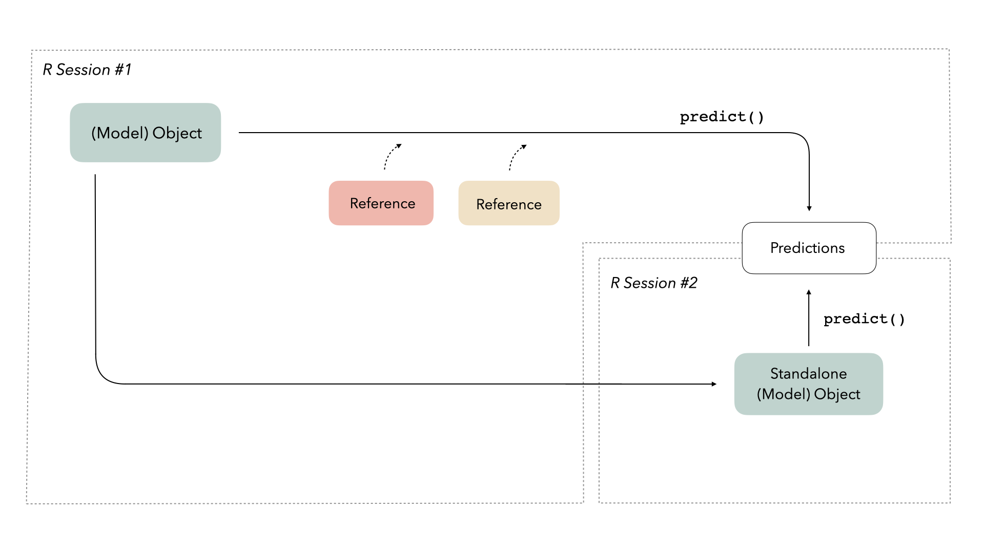
Easy peasy! Now, given that this model is trained, we assume that it’s ready to go to predict on new data. Our mental map might look something like this:

We pass a model object to the predict() function, along with some new data to predict on, and get predictions back. Let’s try that out:

predict(keras_fit, x_test)
#> 1/1 - 0s - 43ms/epoch - 43ms/step
#>            [,1]
#> [1,]  1.4414970
#> [2,]  1.4750962
#> [3,]  0.8539344
#> [4,]  0.5617058
#> [5,] -0.7709445
#> [6,] -1.7506402
#> [7,]  0.9272930

Perfect.

If we’re satisfied with this model and think it provides some valuable insights, we might want to deploy it somewhere—maybe as a REST API or as a Shiny app—so that others can make use of it.

The callr package will be helpful for emulating this kind of situation. The package allows us to start up a fresh R session and pass a few objects in.

We’ll just make use of two of the arguments to the function r():

• func: A function that, given a model object and some new data, will generate predictions, and
• args: A named list, giving the arguments to the above function.

As an example:

r(
  function(x) {
    x * 2
  },
  args = list(
    x = 1
  )
)
#> [1] 2

So, our approach might be:

• save our model object
• start up a new R session
• load the model object into the new session
• predict on new data with the loaded model object

First, saving our model object to a file:

temp_file <- tempfile()

saveRDS(keras_fit, file = temp_file)

Now, starting up a fresh R session and predicting on new data:

r(
  function(temp_file, new_data) {
    library(keras)
    
    model_object <- readRDS(file = temp_file)
    
    predict(model_object, new_data)
  },
  args = list(
    temp_file = temp_file,
    new_data = x_test
  )
)
#> Error: ! in callr subprocess.
#> Caused by error in `do.call(object$predict, args)`:
#> ! 'what' must be a function or character string

Oof. Hm.

After a bit of poking around in keras’ documentation, you might come across the keras vignette “Saving and serializing models” at vignette("saving_serializing", package = "keras"). That vignette points us to several functions in the keras package that will allow us to save our model fit in a way that allows it to predict in a new session.

Given this new understanding, we can update our mental map a bit. Some objects require extra information when they’re loaded into new environments in order to do their thing. In this case, this keras model object needs access to additional references in order to predict on new data.

In computer science, these bits of “extra information” are called references. Those references need to persist—or be restored—in new environments in order for the objects that reference them to work well.

These kinds of custom methods to save objects, like the ones that keras provide, are often referred to as native serialization. Methods for native serialization know which references need to be brought along in order for an object to effectively do its thing in a new environment.

Let’s make use of native serialization, then!

Native serialization, and where it falls short

keras’ vignette is really informative in telling us what we ought to do from here; if we save the model with the native serialization rather than saveRDS, we’ll be good to go.

Saving our model object with their methods:

temp_dir <- tempdir()
save_model_tf(keras_fit, filepath = temp_dir)

Now, starting up a fresh R session and predicting on new data:

r(
  function(temp_dir, new_data) {
    library(keras)
    
    model_object <- load_model_tf(filepath = temp_dir)
    
    predict(model_object, new_data)
  },
  args = list(
    temp_dir = temp_dir,
    new_data = x_test
  )
)
#>            [,1]
#> [1,]  1.4414970
#> [2,]  1.4750962
#> [3,]  0.8539344
#> [4,]  0.5617058
#> [5,] -0.7709445
#> [6,] -1.7506402
#> [7,]  0.9272930

Awesome! Making use of their methods, we were able to effectively save our model, load it in a new R session, and predict on new data.

Now let’s consider a new scenario—I’ve heard that xgboost models are super performant, and want to try to productionize those, too. How would we do that?

Based on our workflow just now, we could try to just save it with saveRDS and see if we get an informative error somewhere along the way to predicting in a new R session. Or, maybe a better approach would be to read through their documentation and see if we can find anything related to serialization.

We’ve done the work of figuring that out, and it turns out the interface is a little bit different. You’ll need to make sure the params object persists across sessions, but saveRDS will work by itself if… ah, I’ll stop myself there.

What if we could just use the same function for any R object, and it would just work?

Using bundle

bundle provides a consistent interface to prepare R model objects to be saved and re-loaded. The package provides two functions, bundle() and unbundle(), that take care of all of the minutae of preparing to save and load R objects effectively.

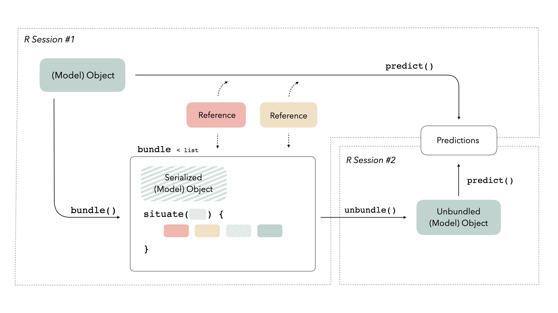
Bundles are just lists with two elements:

• object: The object element of a bundle is the serialized version of the original model object. In the simplest situations in modeling, this object is just the output of a native serialization function like save_model_tf() that we used earlier.
• situate(): The situate() element of a bundle is a function that situates the object element in its new environment. It takes in the object element as input, but also “freezes” reference that existed when the original object was created.

When unbundle() is called on a bundle object, the situate() element of the bundle will re-load the object element and restore needed references in the new environment. Thus, the output of unbundle() is ready to go for prediction wherever it is called.

To be a bit more concrete, lets return to the keras example. Bundling the model fit:

keras_bundle <- bundle(keras_fit)

Now, starting up a fresh R session and predicting on new data:

r(
  function(model_bundle, new_data) {
    library(bundle)
    
    model_object <- unbundle(model_bundle)
 
    predict(model_object, new_data)
  },
  args = list(
    model_bundle = keras_bundle,
    new_data = x_test
  )
)
#>            [,1]
#> [1,]  1.4414970
#> [2,]  1.4750962
#> [3,]  0.8539344
#> [4,]  0.5617058
#> [5,] -0.7709445
#> [6,] -1.7506402
#> [7,]  0.9272930

Huzzah!

The best part is, if you wanted to do the same thing for an xgboost object, you could use the same code!

First, fitting a quick xgboost model:

xgb_fit <- 
  xgboost(
    data = x_train, 
    label = y_train,
    nrounds = 5
  )
#> [1]  train-rmse:0.875983 
#> [2]  train-rmse:0.672900 
#> [3]  train-rmse:0.527715 
#> [4]  train-rmse:0.417273 
#> [5]  train-rmse:0.334283

Now, bundling it:

xgb_bundle <- bundle(xgb_fit)

Now, starting up a fresh R session and predicting on new data:

r(
  function(model_bundle, new_data) {
    library(bundle)
    
    model_object <- unbundle(model_bundle)
    
    predict(model_object, new_data)
  },
  args = list(
    model_bundle = xgb_bundle,
    new_data = x_test
  )
)
#> [1]  1.60800147  0.46607706  0.29694021 -0.05833863  0.24531488
#> [6] -0.76071244  0.29694021

Voilà! We hope bundles are helpful in making your modeling and deployment workflows a good bit smoother in the future.