Transfer learning & fine-tuning

Setup

library(keras3)

Introduction

Transfer learning consists of taking features learned on one problem, and leveraging them on a new, similar problem. For instance, features from a model that has learned to identify raccoon may be useful to kick-start a model meant to identify tanukis.

Transfer learning is usually done for tasks where your dataset has too little data to train a full-scale model from scratch.

The most common incarnation of transfer learning in the context of deep learning is the following workflow:

Take layers from a previously trained model.
Freeze them, so as to avoid destroying any of the information they contain during future training rounds.
Add some new, trainable layers on top of the frozen layers. They will learn to turn the old features into predictions on a new dataset.
Train the new layers on your dataset.

A last, optional step, is fine-tuning, which consists of unfreezing the entire model you obtained above (or part of it), and re-training it on the new data with a very low learning rate. This can potentially achieve meaningful improvements, by incrementally adapting the pretrained features to the new data.

First, we will go over the Keras trainable API in detail, which underlies most transfer learning & fine-tuning workflows.

Then, we’ll demonstrate the typical workflow by taking a model pretrained on the ImageNet dataset, and retraining it on the Kaggle “cats vs dogs” classification dataset.

This is adapted from Deep Learning with Python and the 2016 blog post “building powerful image classification models using very little data”.

Freezing layers: understanding the `trainable` attribute

Layers & models have three weight attributes:

weights is the list of all weights variables of the layer.
trainable_weights is the list of those that are meant to be updated (via gradient descent) to minimize the loss during training.
non_trainable_weights is the list of those that aren’t meant to be trained. Typically they are updated by the model during the forward pass.

Example: the Dense layer has 2 trainable weights (kernel & bias)

layer <- layer_dense(units = 3)
layer$build(shape(NULL, 4))  # Create the weights

length(layer$weights)

## [1] 2

length(layer$trainable_weights)

## [1] 2

length(layer$non_trainable_weights)

## [1] 0

In general, all weights are trainable weights. The only built-in layer that has non-trainable weights is [layer_batch_normalization()]. It uses non-trainable weights to keep track of the mean and variance of its inputs during training. To learn how to use non-trainable weights in your own custom layers, see the guide to writing new layers from scratch.

Example: the BatchNormalization layer has 2 trainable weights and 2 non-trainable weights

layer <- layer_batch_normalization()
layer$build(shape(NA, 4))  # Create the weights

length(layer$weights)

## [1] 4

length(layer$trainable_weights)

## [1] 2

length(layer$non_trainable_weights)

## [1] 2

Layers & models also feature a boolean attribute trainable. Its value can be changed. Setting layer$trainable to FALSE moves all the layer’s weights from trainable to non-trainable. This is called “freezing” the layer: the state of a frozen layer won’t be updated during training (either when training with fit() or when training with any custom loop that relies on trainable_weights to apply gradient updates).

Example: setting trainable to False

layer <- layer_dense(units = 3)
layer$build(shape(NULL, 4))  # Create the weights
layer$trainable <- FALSE  # Freeze the layer

length(layer$weights)

## [1] 2

length(layer$trainable_weights)

## [1] 0

length(layer$non_trainable_weights)

## [1] 2

When a trainable weight becomes non-trainable, its value is no longer updated during training.

# Make a model with 2 layers
layer1 <- layer_dense(units = 3, activation = "relu")
layer2 <- layer_dense(units = 3, activation = "sigmoid")
model <- keras_model_sequential(input_shape = 3) |>
  layer1() |>
  layer2()

# Freeze the first layer
layer1$trainable <- FALSE

# Keep a copy of the weights of layer1 for later reference
# (get_weights() returns a list of R arrays,
#  layer$weights returns a list of KerasVariables)
initial_layer1_weights_values <- get_weights(layer1)

# Train the model
model |> compile(optimizer = "adam", loss = "mse")
model |> fit(random_normal(c(2, 3)), random_normal(c(2, 3)), epochs = 1)

## 1/1 - 0s - 479ms/step - loss: 2.1868

# Check that the weights of layer1 have not changed during training
final_layer1_weights_values <- get_weights(layer1)

all.equal(initial_layer1_weights_values,
          final_layer1_weights_values)

## [1] TRUE

Do not confuse the layer$trainable attribute with the argument training in layer$call() (which controls whether the layer should run its forward pass in inference mode or training mode). For more information, see the Keras FAQ.

Recursive setting of the `trainable` attribute

If you set $trainable <- FALSE on a model or on any layer that has sublayers, all children layers become non-trainable as well.

Example:

inner_model <- keras_model_sequential(input_shape = 3) |>
  layer_dense(units = 3, activation = "relu") |>
  layer_dense(units = 3, activation = "relu")

model <- keras_model_sequential(input_shape = 3) |>
  inner_model() |>
  layer_dense(units = 3, activation = "sigmoid")

model$trainable <- FALSE  # Freeze the outer model

inner_model$trainable  # All layers in `model` are now frozen

## [1] FALSE

inner_model$layers[[1]]$trainable  # `trainable` is propagated recursively

## [1] FALSE

The typical transfer-learning workflow

This leads us to how a typical transfer learning workflow can be implemented in Keras:

Instantiate a base model and load pre-trained weights into it.
Freeze all layers in the base model by setting trainable <- FALSE.
Create a new model on top of the output of one (or several) layers from the base model.
Train your new model on your new dataset.

Note that an alternative, more lightweight workflow could also be:

Instantiate a base model and load pre-trained weights into it.
Run your new dataset through it and record the output of one (or several) layers from the base model. This is called feature extraction.
Use that output as input data for a new, smaller model.

A key advantage of that second workflow is that you only run the base model once on your data, rather than once per epoch of training. So it’s a lot faster & cheaper.

An issue with that second workflow, though, is that it doesn’t allow you to dynamically modify the input data of your new model during training, which is required when doing data augmentation, for instance. Transfer learning is typically used for tasks when your new dataset has too little data to train a full-scale model from scratch, and in such scenarios data augmentation is very important. So in what follows, we will focus on the first workflow.

Here’s what the first workflow looks like in Keras:

First, instantiate a base model with pre-trained weights.

base_model <- application_xception(
  weights = 'imagenet', # Load weights pre-trained on ImageNet.
  input_shape = c(150, 150, 3),
  include_top = FALSE  # Do not include the ImageNet classifier at the top.
)

Then, freeze the base model.

base_model$trainable <- FALSE

Create a new model on top.

inputs <- keras_input(shape = c(150, 150, 3))
# We make sure that the base_model is running in inference mode here,
# by passing `training <- FALSE`. This is important for fine-tuning, as you will
# learn in a few paragraphs.
outputs <- inputs |>
  base_model(training = FALSE) |>
  # Convert features of shape `base_model$output_shape[-1]` to vectors
  layer_global_average_pooling_2d() |>
  # A Dense classifier with a single unit (binary classification)
  layer_dense(1)

model <- keras_model(inputs, outputs)

Train the model on new data.

model |> compile(
  optimizer = optimizer_adam(),
  loss = loss_binary_crossentropy(from_logits = TRUE),
  metrics = list(metric_binary_accuracy())
)
model |> fit(new_dataset, epochs = 20,
             callbacks = ..., validation_data = ...)

Fine-tuning

Once your model has converged on the new data, you can try to unfreeze all or part of the base model and retrain the whole model end-to-end with a very low learning rate.

This is an optional last step that can potentially give you incremental improvements. It could also potentially lead to quick overfitting – keep that in mind.

It is critical to only do this step after the model with frozen layers has been trained to convergence. If you mix randomly-initialized trainable layers with trainable layers that hold pre-trained features, the randomly-initialized layers will cause very large gradient updates during training, which will destroy your pre-trained features.

It’s also critical to use a very low learning rate at this stage, because you are training a much larger model than in the first round of training, on a dataset that is typically very small. As a result, you are at risk of overfitting very quickly if you apply large weight updates. Here, you only want to readapt the pretrained weights in an incremental way.

This is how to implement fine-tuning of the whole base model:

# Unfreeze the base model
base_model$trainable <- TRUE

# It's important to recompile your model after you make any changes
# to the `trainable` attribute of any inner layer, so that your changes
# are take into account
model |> compile(
  optimizer = optimizer_adam(1e-5), # Very low learning rate
  loss = loss_binary_crossentropy(from_logits = TRUE),
  metrics = c(metric_binary_accuracy())
)

# Train end-to-end. Be careful to stop before you overfit!
model |> fit(new_dataset, epochs = 10,
             callbacks = ..., validation_data = ...)

Important note about compile() and trainable

Calling compile() on a model is meant to “freeze” the behavior of that model. This implies that the trainable attribute values at the time the model is compiled should be preserved throughout the lifetime of that model, until compile is called again. Hence, if you change any trainable value, make sure to call compile() again on your model for your changes to be taken into account.

Important notes about BatchNormalization layer

Many image models contain BatchNormalization layers. That layer is a special case on every imaginable count. Here are a few things to keep in mind.

BatchNormalization contains 2 non-trainable weights that get updated during training. These are the variables tracking the mean and variance of the inputs.
When you set bn_layer$trainable <- FALSE, the BatchNormalization layer will run in inference mode, and will not update its mean & variance statistics. This is not the case for other layers in general, as weight trainability & inference/training modes are two orthogonal concepts. But the two are tied in the case of the BatchNormalization layer.
When you unfreeze a model that contains BatchNormalization layers in order to do fine-tuning, you should keep the BatchNormalization layers in inference mode by passing training = FALSE when calling the base model. Otherwise the updates applied to the non-trainable weights will suddenly destroy what the model has learned.

You’ll see this pattern in action in the end-to-end example at the end of this guide.

An end-to-end example: fine-tuning an image classification model on a cats vs. dogs dataset

To solidify these concepts, let’s walk you through a concrete end-to-end transfer learning & fine-tuning example. We will load the Xception model, pre-trained on ImageNet, and use it on the Kaggle “cats vs. dogs” classification dataset.

Getting the data

First, let’s fetch the cats vs. dogs dataset using TFDS. If you have your own dataset, you’ll probably want to use the utility [image_dataset_from_directory()] to generate similar labeled dataset objects from a set of images on disk filed into class-specific folders.

Transfer learning is most useful when working with very small datasets. To keep our dataset small, we will use 40% of the original training data (25,000 images) for training, 10% for validation, and 10% for testing.

# reticulate::py_install("tensorflow-datasets")
tfds <- reticulate::import("tensorflow_datasets")

c(train_ds, validation_ds, test_ds) %<-% tfds$load(
  "cats_vs_dogs",
  # Reserve 10% for validation and 10% for test
  split = c("train[:40%]", "train[40%:50%]", "train[50%:60%]"),
  as_supervised = TRUE  # Include labels
)

length(train_ds)

## [1] 9305

These are the first 9 images in the training dataset – as you can see, they’re all different sizes.

library(tfdatasets, exclude = "shape")

par(mfrow = c(3, 3), mar = c(1,0,1.5,0))
train_ds |>
  dataset_take(9) |>
  as_array_iterator() |>
  iterate(function(batch) {
    c(image, label) %<-% batch
    plot(as.raster(image, max = 255L))
    title(sprintf(
      "label: %s   size: %s",
      label, paste(dim(image), collapse = " x ")))
  })

plot of chunk unnamed-chunk-13

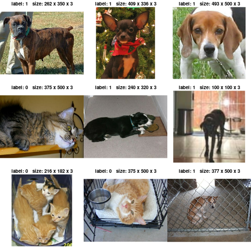
We can also see that label 1 is “dog” and label 0 is “cat”.

Standardizing the data

Our raw images have a variety of sizes. In addition, each pixel consists of 3 integer values between 0 and 255 (RGB level values). This isn’t a great fit for feeding a neural network. We need to do 2 things:

Standardize to a fixed image size. We pick 150x150.
Normalize pixel values between -1 and 1. We’ll do this using a Normalization layer as part of the model itself.

In general, it’s a good practice to develop models that take raw data as input, as opposed to models that take already-preprocessed data. The reason being that, if your model expects preprocessed data, any time you export your model to use it elsewhere (in a web browser, in a mobile app), you’ll need to reimplement the exact same preprocessing pipeline. This gets very tricky very quickly. So we should do the least possible amount of preprocessing before hitting the model.

Here, we’ll do image resizing in the data pipeline (because a deep neural network can only process contiguous batches of data), and we’ll do the input value scaling as part of the model, when we create it.

Let’s resize images to 150x150:

resize_fn <- layer_resizing(width = 150, height = 150)
resize_pair <- function(x, y) list(resize_fn(x), y)

train_ds <- train_ds |> dataset_map(resize_pair)
validation_ds <- validation_ds |> dataset_map(resize_pair)
test_ds <- test_ds |> dataset_map(resize_pair)

Using random data augmentation

When you don’t have a large image dataset, it’s a good practice to artificially introduce sample diversity by applying random yet realistic transformations to the training images, such as random horizontal flipping or small random rotations. This helps expose the model to different aspects of the training data while slowing down overfitting.

data_augmentation <- keras_model_sequential() |>
  layer_random_flip("horizontal") |>
  layer_random_rotation(.1)

train_ds <- train_ds %>%
  dataset_map(function(x, y) list(data_augmentation(x), y))

Let’s batch the data and use prefetching to optimize loading speed.

library(tensorflow, exclude = c("shape", "set_random_seed"))
batch_size <- 64

train_ds <- train_ds |>
  dataset_batch(batch_size) |>
  dataset_prefetch()

validation_ds <- validation_ds |>
  dataset_batch(batch_size) |>
  dataset_prefetch()

test_ds <- test_ds |>
  dataset_batch(batch_size) |>
  dataset_prefetch()

Let’s visualize what the first image of the first batch looks like after various random transformations:

batch <- train_ds |>
  dataset_take(1) |>
  as_iterator() |>
  iter_next()

c(images, labels) %<-% batch
first_image <- images[1, all_dims(), drop = TRUE]
augmented_image <- data_augmentation(first_image, training = TRUE)

plot_image <- function(image, main = deparse1(substitute(image))) {
  image |>
    as.array() |> # convert from tensor to R array
    as.raster(max = 255) |>
    plot()

  if(!is.null(main))
    title(main)
}

par(mfrow = c(2, 2), mar = c(1, 1, 1.5, 1))
plot_image(first_image)
plot_image(augmented_image)
plot_image(data_augmentation(first_image, training = TRUE), "augmented 2")
plot_image(data_augmentation(first_image, training = TRUE), "augmented 3")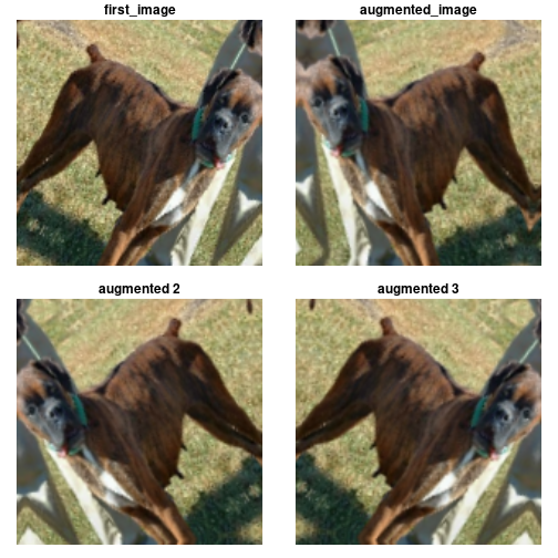

plot of chunk unnamed-chunk-17

Build a model

Now let’s built a model that follows the blueprint we’ve explained earlier.

Note that:

We add a Rescaling layer to scale input values (initially in the [0, 255] range) to the [-1, 1] range.
We add a Dropout layer before the classification layer, for regularization.
We make sure to pass training=FALSE when calling the base model, so that it runs in inference mode, so that batchnorm statistics don’t get updated even after we unfreeze the base model for fine-tuning.

base_model <- application_xception(
  weights = "imagenet", # Load weights pre-trained on ImageNet.
  input_shape = c(150, 150, 3),
  include_top = FALSE, # Do not include the ImageNet classifier at the top.
)

# Freeze the base_model
base_model$trainable <- FALSE

# Create new model on top
inputs <- keras_input(shape = c(150, 150, 3))

# Pre-trained Xception weights requires that input be scaled
# from (0, 255) to a range of (-1., +1.), the rescaling layer
# outputs: `(inputs * scale) + offset`
scale_layer <- layer_rescaling(scale = 1 / 127.5, offset = -1)
x <- scale_layer(inputs)

# The base model contains batchnorm layers. We want to keep them in inference mode
# when we unfreeze the base model for fine-tuning, so we make sure that the
# base_model is running in inference mode here.
outputs <- x |>
  base_model(training = FALSE) |>
  layer_global_average_pooling_2d() |>
  layer_dropout(0.2) |>
  layer_dense(1)

model <- keras_model(inputs, outputs)

summary(model, show_trainable = TRUE)

## Model: "functional_10"
## ┏━━━━━━━━━━━━━━━━━━━━━━━━━━━━━┳━━━━━━━━━━━━━━━━━━━━━━━┳━━━━━━━━━━━━┳━━━━━━━┓
## ┃ Layer (type)                ┃ Output Shape          ┃    Param # ┃ Trai… ┃
## ┡━━━━━━━━━━━━━━━━━━━━━━━━━━━━━╇━━━━━━━━━━━━━━━━━━━━━━━╇━━━━━━━━━━━━╇━━━━━━━┩
## │ input_layer_7 (InputLayer)  │ (None, 150, 150, 3)   │          0 │   -   │
## ├─────────────────────────────┼───────────────────────┼────────────┼───────┤
## │ rescaling (Rescaling)       │ (None, 150, 150, 3)   │          0 │   -   │
## ├─────────────────────────────┼───────────────────────┼────────────┼───────┤
## │ xception (Functional)       │ (None, 5, 5, 2048)    │ 20,861,480 │   N   │
## ├─────────────────────────────┼───────────────────────┼────────────┼───────┤
## │ global_average_pooling2d_1  │ (None, 2048)          │          0 │   -   │
## │ (GlobalAveragePooling2D)    │                       │            │       │
## ├─────────────────────────────┼───────────────────────┼────────────┼───────┤
## │ dropout (Dropout)           │ (None, 2048)          │          0 │   -   │
## ├─────────────────────────────┼───────────────────────┼────────────┼───────┤
## │ dense_8 (Dense)             │ (None, 1)             │      2,049 │   Y   │
## └─────────────────────────────┴───────────────────────┴────────────┴───────┘
##  Total params: 20,863,529 (79.59 MB)
##  Trainable params: 2,049 (8.00 KB)
##  Non-trainable params: 20,861,480 (79.58 MB)

Train the top layer

model |> compile(
  optimizer = optimizer_adam(),
  loss = loss_binary_crossentropy(from_logits = TRUE),
  metrics = list(metric_binary_accuracy())
)

epochs <- 1
model |> fit(train_ds, epochs = epochs, validation_data = validation_ds)

## 146/146 - 40s - 272ms/step - binary_accuracy: 0.9104 - loss: 0.1956 - val_binary_accuracy: 0.9673 - val_loss: 0.0918

Do a round of fine-tuning of the entire model

Finally, let’s unfreeze the base model and train the entire model end-to-end with a low learning rate.

Importantly, although the base model becomes trainable, it is still running in inference mode since we passed training=FALSE when calling it when we built the model. This means that the batch normalization layers inside won’t update their batch statistics. If they did, they would wreck havoc on the representations learned by the model so far.

# Unfreeze the base_model. Note that it keeps running in inference mode
# since we passed `training=FALSE` when calling it. This means that
# the batchnorm layers will not update their batch statistics.
# This prevents the batchnorm layers from undoing all the training
# we've done so far.
base_model$trainable <- TRUE
summary(model, show_trainable = TRUE)

## Model: "functional_10"
## ┏━━━━━━━━━━━━━━━━━━━━━━━━━━━━━┳━━━━━━━━━━━━━━━━━━━━━━━┳━━━━━━━━━━━━┳━━━━━━━┓
## ┃ Layer (type)                ┃ Output Shape          ┃    Param # ┃ Trai… ┃
## ┡━━━━━━━━━━━━━━━━━━━━━━━━━━━━━╇━━━━━━━━━━━━━━━━━━━━━━━╇━━━━━━━━━━━━╇━━━━━━━┩
## │ input_layer_7 (InputLayer)  │ (None, 150, 150, 3)   │          0 │   -   │
## ├─────────────────────────────┼───────────────────────┼────────────┼───────┤
## │ rescaling (Rescaling)       │ (None, 150, 150, 3)   │          0 │   -   │
## ├─────────────────────────────┼───────────────────────┼────────────┼───────┤
## │ xception (Functional)       │ (None, 5, 5, 2048)    │ 20,861,480 │   Y   │
## ├─────────────────────────────┼───────────────────────┼────────────┼───────┤
## │ global_average_pooling2d_1  │ (None, 2048)          │          0 │   -   │
## │ (GlobalAveragePooling2D)    │                       │            │       │
## ├─────────────────────────────┼───────────────────────┼────────────┼───────┤
## │ dropout (Dropout)           │ (None, 2048)          │          0 │   -   │
## ├─────────────────────────────┼───────────────────────┼────────────┼───────┤
## │ dense_8 (Dense)             │ (None, 1)             │      2,049 │   Y   │
## └─────────────────────────────┴───────────────────────┴────────────┴───────┘
##  Total params: 20,867,629 (79.60 MB)
##  Trainable params: 20,809,001 (79.38 MB)
##  Non-trainable params: 54,528 (213.00 KB)
##  Optimizer params: 4,100 (16.02 KB)

model |> compile(
  optimizer = optimizer_adam(1e-5), # Low learning rate
  loss = loss_binary_crossentropy(from_logits = TRUE),
  metrics = list(metric_binary_accuracy())
)

epochs <- 1
model |> fit(train_ds, epochs = epochs, validation_data = validation_ds)

## 146/146 - 79s - 541ms/step - binary_accuracy: 0.8710 - loss: 0.3235 - val_binary_accuracy: 0.9617 - val_loss: 0.1073

After 10 epochs, fine-tuning gains us a nice improvement here. Let’s evaluate the model on the test dataset:

model |> evaluate(test_ds)

## 37/37 - 2s - 42ms/step - binary_accuracy: 0.9557 - loss: 0.1094

## $binary_accuracy
## [1] 0.955718
##
## $loss
## [1] 0.1093767