Understanding the interface to sortable.js
Andrie de Vries and Kenton Russell
2026-02-18
Source:vignettes/understanding_sortable_js.Rmd
understanding_sortable_js.RmdWith the sortable htmlwidget you can
use powerful, dependency-free interactivity from SortableJS
in the browser, RStudio Viewer, or Shiny apps.
The central idea
The key idea to understand about sortable, and
SortableJS in particular, is that the JavaScript will
manipulate an HTML object based on it’s CSS id.
Using sortable in markdown is a little tricky since
markdown does not provide an easy way to provide an id that
we’ll need. We can overcome this by using bare HTML or
using htmltools::tags. Let’s make a simple ul
list. Note, however, that sortable works with nearly any
HTML element, such as div.
An example using raw HTML
The following example uses HTML to construct an unordered list
(<ul>), and then uses sortable_js() to
link the JavaScript required to create interactivity.
Note:
- The HTML
idmatches thecss_idargument ofsortable_js(). - You can drag and drop the list entries. Try it!
<p>You can drag and drop these items in any order (try it!):</p>
<ul id = "example01">
  <li>Move</li>
  <li>Or drag</li>
  <li>Each of the items</li>
  <li>To different positions</li>
</ul>You can drag and drop these items in any order (try it!):
- Move
- Or drag
- Each of the items
- To different positions
Use a tag list to achieve the same, but from R
You can use the functions tags() and
tagList(), both from the htmltools package, to
create HTML.
This means you can construct the sortable list using:
library(htmltools)
tagList(
  tags$ul(
    id = "example02",
    tags$li("drag me"),
    tags$li("sort me"),
    tags$li("any way you like")
  ),
  sortable_js("example02")
)- drag me
- sort me
- any way you like
Little harder but better example
The SortableJS functionality works with any HTML object,
not just lists.
In this next example, you can see how to drag and drop images
(<img>). To embed the plots on the page, you can use
the base64::img() function to encode the png images into a
format that HTML understands.
library(base64enc)
library(withr)

# create two plots for demo purposes
pngfile_1 <- tempfile(fileext = ".png")
with_png(pngfile_1, width = 300, height = 200,{
  plot(1:100, rnorm(100), pch = 21, bg = "red")
  title(main = "Moves Like Jagger")
})

pngfile_2 <- tempfile(fileext = ".png")
with_png(pngfile_2, width = 300, height = 200,{
  barplot(1:9, col = blues9)
  title(main = "I Like the Way You Move")
})
Again, notice that the HTML id matches the
css_id.
tagList(
  tags$div(
    id = "example03",
    tags$image(src = base64enc::dataURI(file = pngfile_1, mime = "image/png")),
    tags$image(src = base64enc::dataURI(file = pngfile_2, mime = "image/png"))
  ),
  sortable_js(css_id = "example03")
)
The power of groups
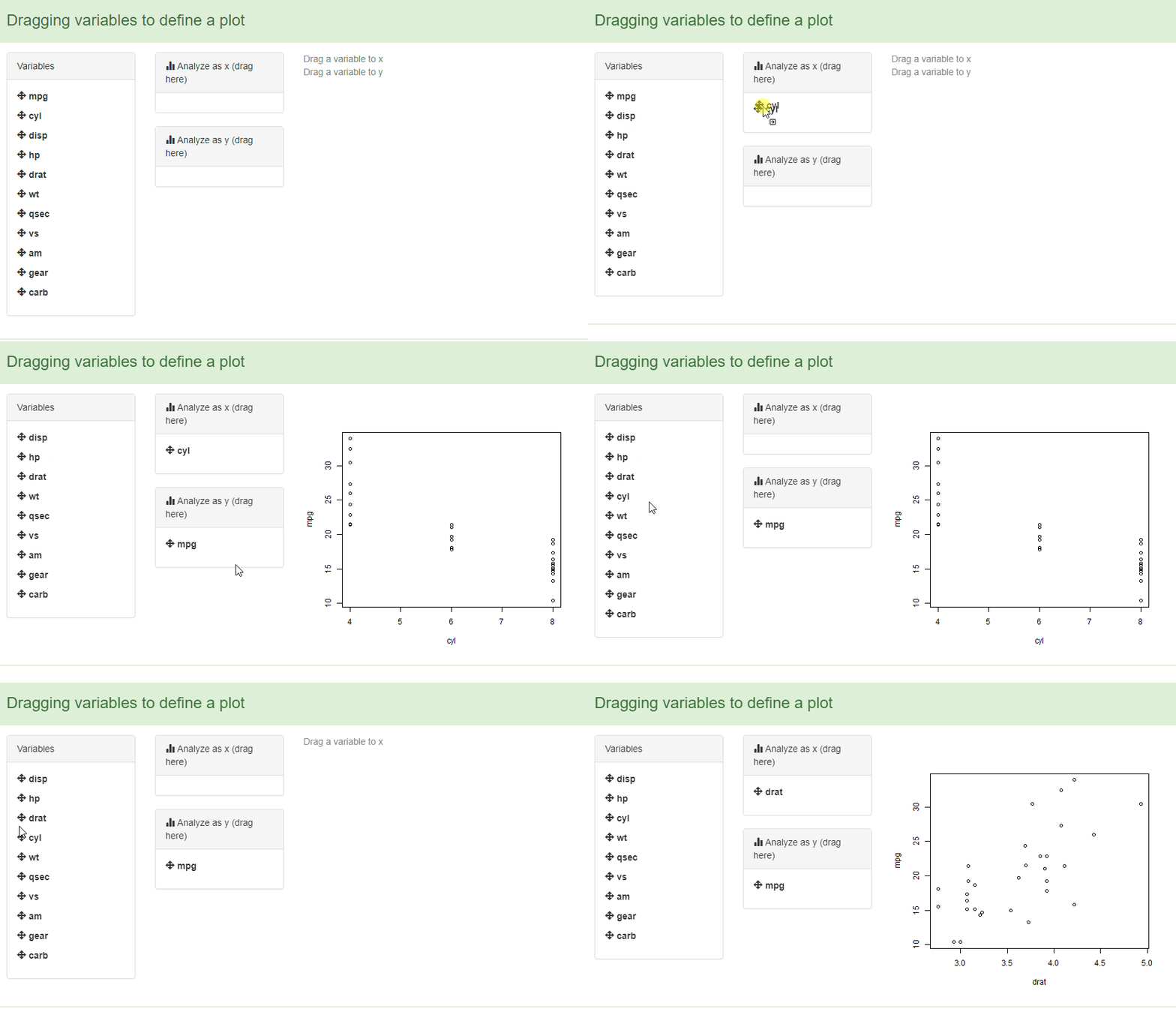
Looking at the SortableJS
excites me about the potential to use sortable as an
important UI element in both a Shiny and non-Shiny context. We could
potentially demo a plot builder with something like this example. You’ll
notice that it doesn’t really do anything, but I hope the intent and
direction is clear.
knitr::read_chunk(
  system.file("shiny/drag_vars_to_plot/app.R", package = "sortable")
)
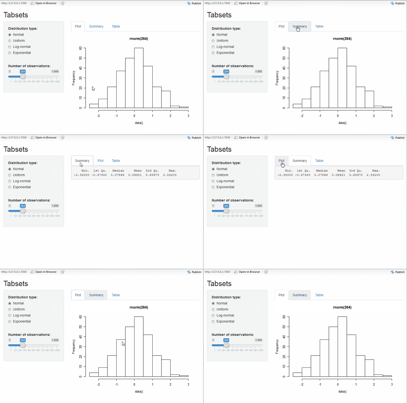
Dragging and dropping shiny tabs
The sortable JS library allows movable tabs inside a
Shiny (and also not Shiny) app.
By adding just one line of code and an id to this RStudio
Tabset
example, you get tabs that the user can re-arrange. You can copy and
paste to see it for yourself, or
runGist("2dbe45f77b65e28acab9").
The modified code snippet is:
# Show a tabset that includes a plot, summary, and table view
# of the generated distribution
mainPanel(
tabsetPanel(
type = "tabs",
id = "sortTab",
tabPanel("Plot", plotOutput("plot")),
tabPanel("Summary", verbatimTextOutput("summary")),
tabPanel("Table", tableOutput("table"))
)
)
),
sortable_js("sortTab")
And the full code:
## Example shiny app to drag-and-drop tabsets in a shiny app


# all credit for code goes to RStudio
# https://github.com/rstudio/shiny/tree/main/006-tabsets
library(sortable)
library(shiny)

ui = # Define UI for random distribution application
  shinyUI(fluidPage(

    # Application title
    titlePanel("Tabsets"),

    # Sidebar with controls to select the random distribution type
    # and number of observations to generate. Note the use of the
    # br() element to introduce extra vertical spacing
    sidebarLayout(
      sidebarPanel(
        radioButtons(
          "dist", "Distribution type:",
          c(
            "Normal" = "norm",
            "Uniform" = "unif",
            "Log-normal" = "lnorm",
            "Exponential" = "exp"
          )
        ),
        br(),

        sliderInput(
          "n",
          "Number of observations:",
          value = 500,
          min = 1,
          max = 1000)
      ),

      # Show a tabset that includes a plot, summary, and table view
      # of the generated distribution
      mainPanel(
        tabsetPanel(
          type = "tabs",
          id = "sortTab",
          tabPanel("Plot", plotOutput("plot")),
          tabPanel("Summary", verbatimTextOutput("summary")),
          tabPanel("Table", tableOutput("table"))
        )
      )
    ),
    sortable_js("sortTab")
  ))

server = function(input, output) {

  # Reactive expression to generate the requested distribution.
  # This is called whenever the inputs change. The output
  # functions defined below then all use the value computed from
  # this expression
  data <- reactive({
    dist <- switch(
      input$dist,
      norm = rnorm,
      unif = runif,
      lnorm = rlnorm,
      exp = rexp,
      rnorm
    )

    dist(input$n)
  })

  # Generate a plot of the data. Also uses the inputs to build
  # the plot label. Note that the dependencies on both the inputs
  # and the data reactive expression are both tracked, and
  # all expressions are called in the sequence implied by the
  # dependency graph
  output$plot <- renderPlot({
    dist <- input$dist
    n <- input$n

    hist(data(),
         main=paste('r', dist, '(', n, ')', sep=''))
  })

  # Generate a summary of the data
  output$summary <- renderPrint({
    summary(data())
  })

  # Generate an HTML table view of the data
  output$table <- renderTable({
    data.frame(x = data())
  })

}

shinyApp( ui, server )