Overview of the sass R package

Carson Sievert

2024-03-15

Why Sass?

Sass is the most widely used, feature rich, and stable CSS extension language available. It has become an essential tool in modern web development because of its ability to reduce complexity and increase composability when styling a website. For a basic example, suppose you want to use the same color for multiple styling rules in your website (e.g., hyperlinks and buttons). With CSS, you’d have to repeat that color every time it is used in styling rule, so in a large project, changing at a later point can be tedious and error-prone.

a {
  color: salmon;
}
button {
  background-color: salmon;
}

With Sass, you could store this color in a Sass variable and use it in the styling rules to produce the same CSS, resulting in a single entry point for the color’s value. This simple Sass tool can make CSS styling a lot easier to reason about, making styles a lot easier to customize and maintain.

$main-color: salmon;
a {
  color: $main-color;
}
button {
  background-color: $main-color;
}

Sass variables are not the only Sass tool useful for reducing complexity. For Sass and sass newcomers, this vignette first covers how to use basic Sass tools like variables, mixins, and functions in the sass R package. After the basics, you’ll also learn how to write composable sass that allows users to easily override your styling defaults and developers to include your Sass in their styling projects. You’ll also learn how to control the CSS output (e.g., compress and cache it), and how to use it in shiny & rmarkdown.

By mastering these concepts, you’ll not only be able to leverage the advantages of using Sass over CSS, but you’ll also have the basis needed to develop R interfaces to Sass projects that allow users to easily customize your styling templates without any knowledge of Sass/CSS. For an example, see the bslib R package, which provides a interface to Bootstrap Sass through easy-to-use functions like bs_theme_add_variables().

Sass Basics

Variables

Sass variables are a great mechanism for simplifying and exposing CSS logic to users. To create a variable, assign a value (likely a CSS property value) to a name, then refer to it by name in downstream Sass code. In this minimal example, we create a body-bg variable then use it to generate a single style rule, but as we’ll see later, variables can also be used inside of other arbitrary Sass code (e.g., functions, mixins, etc).

library(sass)
variable <- "$body-bg: red;"
rule <- "body { background-color: $body-bg; }"
sass(input = list(variable, rule))

/* CSS */
body { 
  background-color: red;
}

A more convenient and readable way to create Sass variables in R is to use a named list(). Also, it’s a good idea to add the !default flag after the value since it provides users of your Sass an opportunity to set their own value. We’ll learn more about defaults in layering, but for now, just note that the !default flag says use this value only if that variable isn’t already defined:

user_default <- list("body-bg" = "blue !default")
default <- list("body-bg" = "red !default")
sass(input = list(user_default, default, rule))

/* CSS */
body { 
  background-color: blue;
}

Functions

Sass comes with a variety of built-in functions (i.e., you don’t have to import anything to start using them) which are useful for working with CSS values (colors, numbers, strings, etc). These built-in functions are primarily useful modifying or combining CSS values in such a way that isn’t possible with CSS. Here we use the rgba() to add alpha blending to black and assign the result to a variable.¹

variable <- list("body-bg" = "rgba(black, 0.8)")
sass(input = list(variable, rule))

/* CSS */
body {
  background-color: rgba(0, 0, 0, 0.8);
}

Sass also provides the ability to define your own functions through the @function at-rule. Like functions in most languages, there are four main components to a function definition: (1) the function name, (2) the function argument/inputs (e.g., arg1, arg2), (3) the function body which contains statements (i.e., statement1, statement2, etc.), and finally (4) a return value.

@function name(arg1, arg2) {
  statement1;
  statement2;
  @return value;
}

For an example of where creating your function becomes useful, consider this color-contrast() function, inspired by this SO answer to a common problem that arises when allowing users control over background color of something (e.g., the document body). We’d like to strive for styling rules that are smart enough to overlay white text on a dark colored background and black text on a light colored background. color-contrast() helps us achieve this since, given a dark color, it returns white; and given a light color, it returns black.

@function color-contrast($color) {
  @return if(
    red($color) * 0.299 + green($color) * 0.587 + blue($color) * 0.114 > 186,
    black, white
  );
}

By saving this function to a file named color-contrast.scss, it can then be imported and used in the following way. For a live example of this in action, consider this Shiny app which allows the user to interactively choose a background color and the title’s font color automatically updates to an appropriate color contrast. See here for more on allowing shiny users to influence styling on the page using sass.

sass(
  list(
    variable,
    sass_file("color-contrast.scss"),
    "body {
      background-color: $body-bg;
      color: color-contrast($body-bg);
    }"
  )
)

/* CSS */
body {
  background-color: rgba(0, 0, 0, 0.8);
  color: white;
}

NOTE: bslib::bs_theme() provides it’s own, more sophisticated, version of color-contrast() that you can use like so: sass::sass_partial("body{color: color-contrast($body-bg)}", bs_theme())

Importing

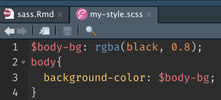
In practice, you’ll want to write your Sass code in .scss (or .sass) files (instead of inside R strings). That way you can leverage things like syntax highlighting in RStudio (or your favorite IDE) and make it easier for others to import your Sass into their workflow. For example, if I have .scss file in my working directory, say my-style.scss, I can compile it this way:

sass(sass_file("my-style.scss"))

/* CSS */
body {
  background-color: rgba(0, 0, 0, 0.8);
}

This works because sass_file() uses sass_import() to generate an @import at-rule. If you visit the docs for @import, you’ll notice there’s more you can do that import local .scss, like import local or remote .css files, import font files, and more. Note also that sass also provides tools that make importing of local font files easier – see font_google() to learn more.

Font imports

Importing font file(s) directly in Sass/CSS/HTML can be a headache to implement. This is especially true if you want to serve font files so that a custom font renders on any client machine, even if the client is without an internet connection. To make this easier, sass provides a font_google() which can be used to download, cache, import, and serve the relevant font files all at once.

library(htmltools)

my_font <- list("my-font" = font_google("Pacifico"))
css <- sass(
  list(
    my_font,
    list("body {font-family: $my-font}")
  )
)

shinyApp(
  fluidPage(
    "Hello",
    tags$style(css)
  ), 
  function(...) {}
)

To import non-Google fonts, use either font_link() or font_face(). The former is for importing fonts via a remote URL whereas the former could be use to import any font locally (or remotely).

Mixins

Similar to how functions are useful for encapsulating computation in a reusable unit, mixins are useful for doing the same with styling rules (i.e., packaging them into a reusable unit). Technically speaking, mixins are similar to functions in that they require a name, may have arguments, as well as any number of statements. However, they differ in that they require the return value to be a style rule, and when called, need to be @included in a larger style rule in order to generate any CSS.

For some examples, please see the Sass mixin documentation.

More basics

This vignette intentionally doesn’t try to re-invent the existing and wonderful Sass documentation. There you’ll find many more useful things as you start to write more Sass, such as control flow, lists, maps, interpolation, and more.

Composable sass

To make Sass code more composable with other Sass code (e.g., allowing others to change your variable defaults or import a function or mixin you’ve defined), consider partitioning your Sass code into a sass::sass_layer(). The main idea is to split your Sass into 4 parts: functions, defaults (i.e. variable defaults), mixins, and rules (i.e., styling rules).

layer1 <- sass_layer(
  functions = sass_file("color-contrast.scss"),
  defaults = list("body-bg" = "black !default"),
  rules = "body{background-color: $body-bg; color: color-contrast($body-bg)}"
)
as_sass(layer1)

/* CSS */
body {
  background-color: black;
  color: white;
}

This allows downstream sass_layer()s to be sass_bundle()d into a single layer, where defaults in downstream layers are granted higher priority. More specifically, this means:

• defaults for layer2 are placed before defaults for layer1.
  • Allowing downstream Sass to override variable defaults in upstream Sass.
• rules for layer2 are placed after rules for layer1.
  • Allows downstream rules to take precedence over upstream rules (precedence matters when there are multiple rules with the same level of specificity).

layer2 <- sass_layer(
  defaults = list("body-bg" = "white !default")
)
sass(sass_bundle(layer1, layer2))

/* CSS */
body {
  background-color: white;
  color: black;
}

Resolving relative imports

Another problem that sass_layer() helps solve is that sometimes your Sass code might want to import a local file using a relative path that you know how to resolve, but not necessarily the person who eventually compiles your Sass. To solve this issue, provide a named character vector to file_attachments, pointing the relevant relative path(s) to the appropriate absolute path(s). Here’s a contrived example of how that might look (here’s a more real example of using it in an R package).

sass_layer(
  declarations = "@import url('fonts/Source_Sans_Pro_300.ttf')",
  file_attachments = c(
    fonts = '/full/path/to/my/local/fonts'
  )
)

Attaching HTML dependencies

Another problem that sass_layer() helps solve is that sometimes you want to attach other HTML dependencies to your Sass/CSS (e.g., JavaScript, other CSS, etc). For this reason, sass_layer() has a html_deps argument to which you can provide htmltools::htmlDependency() objects. sass() preserves these, as well as any other HTML dependencies attached to it’s input, by including them in the return value. This ensures that, when you include sass() in rmarkdown or shiny those dependencies come along for the ride.

DISCLAIMER: If you want to use this feature and include CSS as a file in shiny, you’ll need to call htmltools::htmlDependencies() on the return value of sass() to get the dependencies, then include them in your user interface definition.

CSS output options

The sass() function provides a few arguments for controlling the CSS output it generates, including output, options, and cache_options. The following covers some of the most important options available.

Output to a file

If the CSS generated from sass() can be useful in more than one place, consider writing it to a file (instead of returning it as a string). To write CSS to a file, give a suitable file path to sass()’s output argument.

sass(
  sass_file("my-style.scss"),
  output = "my-style.css"
)

Compression

By default, sass() outputs 'expanded' CSS meaning there are lots of white-space and line-breaks included to make it more readable by humans. Computers don’t need all those unnecessary characters, so to speed up your page load time when you go to include the CSS in shiny or rmarkdown, consider removing them altogether with output_style = "compressed":

sass(
  sass_file("my-style.scss"),
  options = sass_options(output_style = "compressed")
)

Source maps

When compressing the CSS output, it can be useful to include a source map so that it’s easier to inspect the CSS from the website. The easiest way to include a source map is to set source_map_embed = TRUE:

sass(
  sass_file("my-style.scss"),
  options = sass_options(
    output_style = "compressed",
    source_map_embed = TRUE
  )
)

Caching

Sometimes calling sass() can be computationally expensive, in which case, it can be useful to leverage its caching capability. Caching is enabled by default, unless Shiny’s Developer Mode (shiny::devmode()) is enabled. To explicitly enable (disable), set options(sass.cache = ) to TRUE (or FALSE):

withr::with_options(
  list(sass.cache = TRUE),
  sass(sass_file("my-style.scss"))
)

You can also configure the location, size, and age of file caching via sass_file_cache(), which can be passed directly to a sass() call:

sass(
  sass_file("my-style.scss"),
  cache = sass_file_cache(getwd(), max_size = 100 * 1024^2)
)

Or used with sass_cache_set_dir() to configure the file cache globally:

sass_cache_set_dir(getwd(), sass_file_cache(getwd(), max_size = 100 * 1024^2))

Note that the location of the file cache defaults to sass_cache_context_dir(), which depends on the context in which it’s running. When inside a Shiny app, the cache location is relative to the app’s directory so the cache can persist and be shared across R processes. Otherwise, the context directory is a OS and package specific caching directory.

In shiny

There are two basic approaches to including the CSS that sass() returns as HTML in your shiny app. If you’re curious, the official shiny article on CSS has more details with a couple different approaches. Regardless of the approach, consider leveraging compressing and caching the CSS output to make your app faster to load.

As a string

The character string that sass() returns is already marked as HTML()², so to include it in your shiny app, wrap it in a <style> tag. It’s not necessary to place this tag in the <head> of the document, but it’s good practice:

library(shiny)
css <- sass(sass_file("my-style.scss"))
fluidPage(
  tags$head(tags$style(css),
  ...
)

As a file

To write CSS to a file, give a suitable file path to sass()’s output argument. Here we write to a specially named www/ subdirectory so that shiny will automatically make those file(s) available to the web app.

library(shiny)
sass(
  sass_file("my-style.scss"),
  output = "www/my-style.css"
)
fluidPage(
  tags$head(
    tags$link(href = "my-style.css", rel = "stylesheet", type = "text/css")
  ),
  ...
)

As a dynamic input

Sometimes it’s useful to allow users of your shiny app to be able to influence your app’s styling via shiny input(s). One way this can be done is via dynamic UI, where you use renderUI()/uiOutput() to dynamically insert CSS as an HTML string whenever a relevant input changes. Be aware, however, that whenever you allow dynamic user input to generate HTML(), you’re leaving yourself open to security vulnerabilites; so try to avoid it, and never allow clients to enter free form textInput() without any sort of sanitation of the user input.

Consider this basic example of using a colourInput() widget (from the colourpicker package) to choose the body’s background color, which triggers a call to sass():

library(shiny)

ui <- fluidPage(
  headerPanel("Sass Color Example"),
  colourpicker::colourInput("color", "Background Color", value = "#6498d2", showColour = "text"),
  uiOutput("sass")
)

server <- function(input, output) {
  output$sass <- renderUI({
    tags$head(tags$style(css()))
  })
  css <- reactive({
    sass::sass(list(
      list(color = input$color),
      "body { background-color: $color; }"
    ))
  })
}

shinyApp(ui, server)

Below are a few more sophisticated examples of dynamic input:

• Font Color
  • https://gallery.shinyapps.io/sass-font
  • shiny::runApp(system.file("sass-font", package = "sass"))
• Sizing
  • https://gallery.shinyapps.io/sass-size
  • shiny::runApp(system.file("sass-size", package = "sass"))
• Themes
  • https://gallery.shinyapps.io/sass-theme
  • shiny::runApp(system.file("sass-theme", package = "sass"))

In rmarkdown

knitr recently gained a Sass engine powered by the sass package. This means you can write Sass code directly into a code sass chunk and the resulting CSS will be included in the resulting document (The echo = FALSE prevents the Sass code from being shown in the resulting document).

```{sass, echo = FALSE}
$body-bg: red;
body{
  background-color: $body-bg;
}
```

If you like to write R sass code instead, you can do that as well, and by default it works similarly to the sass engine (except that the sass-specific code chunk options will be ignored, but you can specify those options via sass::sass() instead).

```{r, echo = FALSE}
sass(sass_file("my-style.scss"))
```

If syntax highlighting is enabled in your output document , it’s also possible to display the generated CSS (instead of embedding it as HTML) with syntax highlighting by setting the code chunk options class.output='css' and comment=''. Unfortunately, for some output formats, like rmarkdown::html_vignette(), syntax hightlighting isn’t supported, but for output formats like rmarkdown::html_document(), you can enable syntax highlighting by setting the highlight parameter to a non-default value (e.g., tango).

```{r, class.output='css', comment=''}
sass(sass_file("my-style.scss"))
```

---

1. Oh, by the way, the value of a variable may be an expression.↩︎

2. Including dynamic user input directly as HTML(), especially with free form inputs like textInput(), is a security vulnerability. Avoid it if you can.↩︎