Uncertainty estimates with layer_dense_variational

With tfprobability, we can compute uncertainty estimates for keras layers. This vignette shows how to do this for dense layers.

Our example will have two types of uncertainty estimated:

that due to variation in the data (irreducible; a.k.a. aleatoric)
that due to the fact that we don’t know the true model (theoretically, minimizable in the limit of infinite data, a.k.a. epistemic)

To achieve the former, we have our model learn the spread in the data; to achieve the latter, we use a variational layer that learns a posterior over the weights. Internally, this layer works by minimizing the evidence lower bound (ELBO), thus striving to find an approximative posterior that does two things:

fit the actual data well (put differently: achieve high log likelihood), and
stay close to a prior (as measured by KL divergence).

As users, we get to specify the form of the posterior as well as that of the prior. But first let’s generate some data.

library(tensorflow)
# assume it's version 1.14, with eager not yet being the default
tf$compat$v1$enable_v2_behavior()

library(tfprobability)
library(keras)

library(dplyr)
library(tidyr)
library(ggplot2)

# generate the data
x_min <- -40
x_max <- 60
n <- 150
w0 <- 0.125
b0 <- 5

normalize <- function(x) (x - x_min) / (x_max - x_min)

# training data; predictor 
x <- x_min + (x_max - x_min) * runif(n) %>% as.matrix()

# training data; target
eps <- rnorm(n) * (3 * (0.25 + (normalize(x)) ^ 2))
y <- (w0 * x * (1 + sin(x)) + b0) + eps

# test data (predictor)
x_test <- seq(x_min, x_max, length.out = n) %>% as.matrix()

ggplot(data.frame(x = x, y = y), aes(x, y)) + geom_point()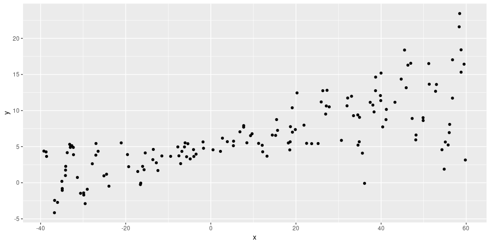

Simulated data

Here is a simple, trainable prior (in empirical Bayesian spirit: A normal distribution where the network may learn the mean (but not the scale). Alternatively, we could disallow learning from the data by setting trainable to FALSE.

prior_trainable <-
  function(kernel_size,
           bias_size = 0,
           dtype = NULL) {
    n <- kernel_size + bias_size
    keras_model_sequential() %>%
      layer_variable(n, dtype = dtype, trainable = TRUE) %>%
      layer_distribution_lambda(function(t) {
        tfd_independent(tfd_normal(loc = t, scale = 1),
                        reinterpreted_batch_ndims = 1)
      })
  }

The posterior then is a normal, too:

posterior_mean_field <-
  function(kernel_size,
           bias_size = 0,
           dtype = NULL) {
    n <- kernel_size + bias_size
    c <- log(expm1(1))
    keras_model_sequential(list(
      layer_variable(shape = 2 * n, dtype = dtype),
      layer_distribution_lambda(
        make_distribution_fn = function(t) {
          tfd_independent(tfd_normal(
            loc = t[1:n],
            scale = 1e-5 + tf$nn$softplus(c + t[(n + 1):(2 * n)])
            ), reinterpreted_batch_ndims = 1)
        }
      )
    ))
  }

Now for the main model. The variational-dense layer is defined to have two units, one for the distribution of means and distribution of scales each. layer_distribution_lambda then takes their respective outputs as the mean and scale of the posterior distribution.

model <- keras_model_sequential() %>%
  layer_dense_variational(
    units = 2,
    make_posterior_fn = posterior_mean_field,
    make_prior_fn = prior_trainable,
    # scale by the size of the dataset
    kl_weight = 1 / n
  ) %>%
  layer_distribution_lambda(function(x)
    tfd_normal(loc = x[, 1, drop = FALSE],
               scale = 1e-3 + tf$math$softplus(0.01 * x[, 2, drop = FALSE])
               )
    )

The model is then simply trained to minimize the negative log likelihood, and fitted like a normal keras network.

negloglik <- function(y, model) - (model %>% tfd_log_prob(y))
model %>% compile(optimizer = optimizer_adam(lr = 0.01), loss = negloglik)
model %>% fit(x, y, epochs = 1000)

Because of the uncertainty in the weights, this model does not predict one line, but an ensemble of lines. Each of these lines has its own opinion about the spread in the data. Here is a way we could display this – each colored line is the mean of a distribution, surrounded by a confidence band indicating +/- two standard deviations.

# each time we ask the model to predict, we get a different line
yhats <- purrr::map(1:100, function(x) model(tf$constant(x_test)))
means <-
  purrr::map(yhats, purrr::compose(as.matrix, tfd_mean)) %>% abind::abind()
sds <-
  purrr::map(yhats, purrr::compose(as.matrix, tfd_stddev)) %>% abind::abind()

means_gathered <- data.frame(cbind(x_test, means)) %>%
  gather(key = run, value = mean_val,-X1)
sds_gathered <- data.frame(cbind(x_test, sds)) %>%
  gather(key = run, value = sd_val,-X1)

lines <-
  means_gathered %>% inner_join(sds_gathered, by = c("X1", "run"))
mean <- apply(means, 1, mean)

ggplot(data.frame(x = x, y = y, mean = as.numeric(mean)), aes(x, y)) +
  geom_point() +
  theme(legend.position = "none") +
  geom_line(aes(x = x_test, y = mean), color = "violet", size = 1.5) +
  geom_line(
    data = lines,
    aes(x = X1, y = mean_val, color = run),
    alpha = 0.6,
    size = 0.5
  ) +
  geom_ribbon(
    data = lines,
    aes(
      x = X1,
      ymin = mean_val - 2 * sd_val,
      ymax = mean_val + 2 * sd_val,
      group = run
    ),
    alpha = 0.05,
    fill = "grey",
    inherit.aes = FALSE
  )

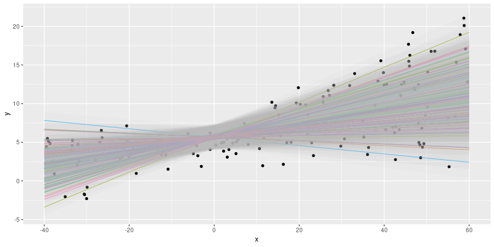
Displaying both epistemic and aleatoric uncertainty on the simulated dataset.

Summing up, using layer_dense_variational we are able to construct a posterior predictive distribution from an ensemble of models, where each single model by itself learns the spread in the data. For some more background narrative on this topic, see Adding uncertainty estimates to Keras models with tfprobability.

Sigrid Keydana

2021-05-20