Dynamic linear models

In state space models, we assume that there is a latent process, hidden from our eyes; all we have are the observations we can make. The process evolves due to some hidden logic (transition model); and the way it produces the observations follows some hidden logic (observation model). There is noise in process evolution, and there is noise in observation. If the transition and observation models both are linear, and the process as well as observation noise are Gaussian, we have a linear-Gaussian state space model (SSM). The task then is to infer the latent state from the observations. The most famous technique here is the Kálmán filter.

In practical applications, two characteristics of linear-Gaussian SSMs are especially attractive.

For one, they let us estimate dynamically changing parameters. In regression, the parameters can be viewed as a hidden state; we may thus have a slope and an intercept that vary over time. When parameters can vary, we speak of dynamic linear models (DLMs). In this vignette, we introduce DLMs by way of dynamic linear regression.

Second, linear-Gaussian SSMs are useful in time-series forecasting because Gaussian processes can be added. A time series can thus be framed as, e.g. the sum of a linear trend and a process that varies seasonally. At the end of the vignette, we refer to a post that illustrates this application.

For the walkthrough of dynamic linear regression, we use an example by Petris et al.(2009), Dynamic linear models with R. The example applies dynamic regression to the Capital Asset Pricing Model (CAPM) data from Berndt (1991). This dataset has monthly returns, collected from January 1978 to December 1987, for four different stocks, the 30-day Treasury Bill – standing in for a risk-free asset –, and the value-weighted average returns for all stocks listed at the New York and American Stock Exchanges, representing the overall market returns.

library(tensorflow)
library(tfprobability)

library(tidyverse)
library(zeallot)

# As the data does not seem to be available at the address given in Petris et al. any more,
# we put it on the TensorFlow for R blog for download
# download from:
# https://github.com/rstudio/ai-blog/tree/master/_posts/2019-06-25-dynamic_linear_models_tfprobability/data/capm.txt
df <- read_table(
  "capm.txt",
  col_types = list(X1 = col_date(format = "%Y.%m"))) %>%
  rename(month = X1)
df %>% glimpse()

Observations: 120
Variables: 7
$ month  <date> 1978-01-01, 1978-02-01, 1978-03-01, 1978-04-01, 1978-05-01, 19…
$ MOBIL  <dbl> -0.046, -0.017, 0.049, 0.077, -0.011, -0.043, 0.028, 0.056, 0.0…
$ IBM    <dbl> -0.029, -0.043, -0.063, 0.130, -0.018, -0.004, 0.092, 0.049, -0…
$ WEYER  <dbl> -0.116, -0.135, 0.084, 0.144, -0.031, 0.005, 0.164, 0.039, -0.0…
$ CITCRP <dbl> -0.115, -0.019, 0.059, 0.127, 0.005, 0.007, 0.032, 0.088, 0.011…
$ MARKET <dbl> -0.045, 0.010, 0.050, 0.063, 0.067, 0.007, 0.071, 0.079, 0.002,…
$ RKFREE <dbl> 0.00487, 0.00494, 0.00526, 0.00491, 0.00513, 0.00527, 0.00528, …

The Capital Asset Pricing Model then assumes a linear relationship between the excess returns of an asset under study and the excess returns of the market. For both, excess returns are obtained by subtracting the returns of the chosen risk-free asset; then, the scaling coefficient between them reveals the asset to either be an “aggressive” investment (slope > 1: changes in the market are amplified), or a conservative one (slope < 1: changes are damped).

Assuming this relationship does not change over time, we can easily use lm to illustrate this. Following Petris et al. in zooming in on IBM as the asset under study, we have

# excess returns of the asset under study
ibm <- df$IBM - df$RKFREE
# market excess returns
x <- df$MARKET - df$RKFREE

fit <- lm(ibm ~ x)
summary(fit)

Call:
lm(formula = ibm ~ x)

Residuals:
     Min       1Q   Median       3Q      Max 
-0.11850 -0.03327 -0.00263  0.03332  0.15042 

Coefficients:
              Estimate Std. Error t value Pr(>|t|)    
(Intercept) -0.0004896  0.0046400  -0.106    0.916    
x            0.4568208  0.0675477   6.763 5.49e-10 ***
---
Signif. codes:  0 ‘***’ 0.001 ‘**’ 0.01 ‘*’ 0.05 ‘.’ 0.1 ‘ ’ 1

Residual standard error: 0.05055 on 118 degrees of freedom
Multiple R-squared:  0.2793,    Adjusted R-squared:  0.2732 
F-statistic: 45.74 on 1 and 118 DF,  p-value: 5.489e-10

So IBM is found to be a conservative investment, the slope being ~ 0.5. But is this relationship stable over time?

Let’s turn to tfprobability to investigate.

# zoom in on ibm
ts <- ibm %>% matrix()
# forecast 12 months
n_forecast_steps <- 12
ts_train <- ts[1:(length(ts) - n_forecast_steps), 1, drop = FALSE]

# make sure we work with float32 here
ts_train <- tf$cast(ts_train, tf$float32)
ts <- tf$cast(ts, tf$float32)

In consttructing the model, sts_dynamic_linear_regression() does what we want:

# define the model on the complete series
linreg <- ts %>%
  sts_dynamic_linear_regression(
    design_matrix = cbind(rep(1, length(x)), x) %>% tf$cast(tf$float32)
  )

Now we define a function, fit_with_vi, that

trains the model on the training set, using variational inference (sts_build_factored_variational_loss())
obtains forecasts using sts_forecast()
obtains the smoothed as well as the filtered estimates from the Kálmán Filter by converting to a tfd_linear_gaussian_state_space_model() and calling posterior_marginals() on it:

fit_with_vi <-
  function(ts,
           ts_train,
           model,
           n_iterations,
           n_param_samples,
           n_forecast_steps,
           n_forecast_samples) {
    
    optimizer <- tf$compat$v1$train$AdamOptimizer(0.1)
    
    loss_and_dists <-
      ts_train %>% sts_build_factored_variational_loss(model = model)
    variational_loss <- loss_and_dists[[1]]
    train_op <- optimizer$minimize(variational_loss)
    
    with (tf$Session() %as% sess,  {
      
      # step 1: train the model using variational inference
      sess$run(tf$compat$v1$global_variables_initializer())
      for (step in 1:n_iterations) {
        sess$run(train_op)
        loss <- sess$run(variational_loss)
        if (step %% 1 == 0)
          cat("Loss: ", as.numeric(loss), "\n")
      }
      # step 2: obtain forecasts
      variational_distributions <- loss_and_dists[[2]]
      posterior_samples <-
        Map(
          function(d)
            d %>% tfd_sample(n_param_samples),
          variational_distributions %>% reticulate::py_to_r() %>% unname()
        )
      forecast_dists <-
        ts_train %>% sts_forecast(model, posterior_samples, n_forecast_steps)
      fc_means <- forecast_dists %>% tfd_mean()
      fc_sds <- forecast_dists %>% tfd_stddev()
      
      # step 3: obtain smoothed and filtered estimates from the Kálmán filter
      ssm <- model$make_state_space_model(length(ts_train), param_vals = posterior_samples)
      c(smoothed_means, smoothed_covs) %<-% ssm$posterior_marginals(ts_train)
      c(., filtered_means, filtered_covs, ., ., ., .) %<-% ssm$forward_filter(ts_train)
   
      c(posterior_samples, fc_means, fc_sds, smoothed_means, smoothed_covs, filtered_means, filtered_covs) %<-%
        sess$run(list(posterior_samples, fc_means, fc_sds, smoothed_means, smoothed_covs, filtered_means, filtered_covs))
      
    })
    
    list(
      variational_distributions,
      posterior_samples,
      fc_means[, 1],
      fc_sds[, 1],
      smoothed_means,
      smoothed_covs,
      filtered_means,
      filtered_covs
    )
  }

Now we’re ready to call that function.

# number of VI steps
n_iterations <- 300
# sample size for posterior samples
n_param_samples <- 50
# sample size to draw from the forecast distribution
n_forecast_samples <- 50

# call fit_vi defined above
c(
  param_distributions,
  param_samples,
  fc_means,
  fc_sds,
  smoothed_means,
  smoothed_covs,
  filtered_means,
  filtered_covs
) %<-% fit_vi(
  ts,
  ts_train,
  model,
  n_iterations,
  n_param_samples,
  n_forecast_steps,
  n_forecast_samples
)

Let’s look at the forecasts and filtering resp. smoothing estimates.

Putting all we need into one dataframe, we have

smoothed_means_intercept <- smoothed_means[, , 1] %>% colMeans()
smoothed_means_slope <- smoothed_means[, , 2] %>% colMeans()

smoothed_sds_intercept <- smoothed_covs[, , 1, 1] %>% colMeans() %>% sqrt()
smoothed_sds_slope <- smoothed_covs[, , 2, 2] %>% colMeans() %>% sqrt()

filtered_means_intercept <- filtered_means[, , 1] %>% colMeans()
filtered_means_slope <- filtered_means[, , 2] %>% colMeans()

filtered_sds_intercept <- filtered_covs[, , 1, 1] %>% colMeans() %>% sqrt()
filtered_sds_slope <- filtered_covs[, , 2, 2] %>% colMeans() %>% sqrt()

forecast_df <- df %>%
  select(month, IBM) %>%
  add_column(pred_mean = c(rep(NA, length(ts_train)), fc_means)) %>%
  add_column(pred_sd = c(rep(NA, length(ts_train)), fc_sds)) %>%
  add_column(smoothed_means_intercept = c(smoothed_means_intercept, rep(NA, n_forecast_steps))) %>%
  add_column(smoothed_means_slope = c(smoothed_means_slope, rep(NA, n_forecast_steps))) %>%
  add_column(smoothed_sds_intercept = c(smoothed_sds_intercept, rep(NA, n_forecast_steps))) %>%
  add_column(smoothed_sds_slope = c(smoothed_sds_slope, rep(NA, n_forecast_steps))) %>%
  add_column(filtered_means_intercept = c(filtered_means_intercept, rep(NA, n_forecast_steps))) %>%
  add_column(filtered_means_slope = c(filtered_means_slope, rep(NA, n_forecast_steps))) %>%
  add_column(filtered_sds_intercept = c(filtered_sds_intercept, rep(NA, n_forecast_steps))) %>%
  add_column(filtered_sds_slope = c(filtered_sds_slope, rep(NA, n_forecast_steps)))

Here first are the forecasts.

ggplot(forecast_df, aes(x = month, y = IBM)) +
  geom_line(color = "grey") +
  geom_line(aes(y = pred_mean), color = "cyan") +
  geom_ribbon(
    aes(ymin = pred_mean - 2 * pred_sd, ymax = pred_mean + 2 * pred_sd),
    alpha = 0.2,
    fill = "cyan"
  ) +
  theme(axis.title = element_blank())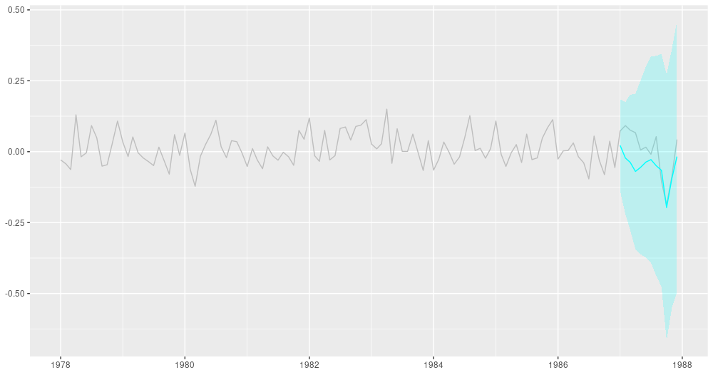

12-point-ahead forecasts for IBM; posterior means +/- 2 standard deviations.

Here are the smoothing estimates. The intercept (shown in orange) remains pretty stable over time, but we do see a trend in the slope (displayed in green).

ggplot(forecast_df, aes(x = month, y = smoothed_means_intercept)) +
  geom_line(color = "orange") +
  geom_line(aes(y = smoothed_means_slope),
            color = "green") +
  geom_ribbon(
    aes(
      ymin = smoothed_means_intercept - 2 * smoothed_sds_intercept,
      ymax = smoothed_means_intercept + 2 * smoothed_sds_intercept
    ),
    alpha = 0.3,
    fill = "orange"
  ) +
  geom_ribbon(
    aes(
      ymin = smoothed_means_slope - 2 * smoothed_sds_slope,
      ymax = smoothed_means_slope + 2 * smoothed_sds_slope
    ),
    alpha = 0.1,
    fill = "green"
  ) +
  coord_cartesian(xlim = c(forecast_df$month[1], forecast_df$month[length(ts) - n_forecast_steps]))  +
  theme(axis.title = element_blank())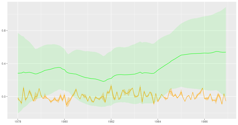

Smoothing estimates from the Kálmán filter. Green: coefficient for dependence on excess market returns (slope), orange: vector of ones (intercept).

For comparison, this is how the filtered estimates look.

ggplot(forecast_df, aes(x = month, y = filtered_means_intercept)) +
  geom_line(color = "orange") +
  geom_line(aes(y = filtered_means_slope),
            color = "green") +
  geom_ribbon(
    aes(
      ymin = filtered_means_intercept - 2 * filtered_sds_intercept,
      ymax = filtered_means_intercept + 2 * filtered_sds_intercept
    ),
    alpha = 0.3,
    fill = "orange"
  ) +
  geom_ribbon(
    aes(
      ymin = filtered_means_slope - 2 * filtered_sds_slope,
      ymax = filtered_means_slope + 2 * filtered_sds_slope
    ),
    alpha = 0.1,
    fill = "green"
  ) +
  coord_cartesian(ylim = c(-2, 2),
                  xlim = c(forecast_df$month[1], forecast_df$month[length(ts) - n_forecast_steps])) +
  theme(axis.title = element_blank())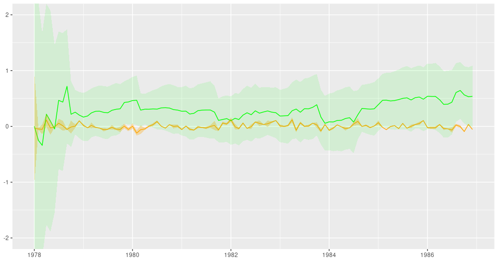

Filtering estimates from the Kálmán filter. Green: coefficient for dependence on excess market returns (slope), orange: vector of ones (intercept).

For an example illustrating the additivity feature of DLMs – that allows us to decompose a time series into its constituents –, as well as for more narrative on the above example, see Dynamic linear models with tfprobability on the TensorFlow for R blog.

Sigrid Keydana

2021-05-20