Advanced Information Management

In the Intro to Information Management article, we learned all about how to synthesize information on a table, giving us a useful report that can be published and widely shared. We used a pointblank informant with a set of information functions to generate info text and put that text into the appropriate report sections. We’re going to take this a few steps further and look into some more functionality makes info text more dynamic and also include a finalizing step in this workflow that accounts for evolving data.

Getting Snippets of Useful Text With the info_snippet() Function

A great source of information about the table can be the table itself. Suppose you want to show some categorical values from a particular column. Maybe you’d like to display the range of values in an important numeric column. Perhaps show some KPI values that can be calculated using data in the table? This can all be done with the info_snippet() function. You give the snippet a name and you give it a function call. Let’s do this for the small_table dataset available in pointblank. This is what that table looks like:

small_table

## # A tibble: 13 × 8
##    date_time           date           a b             c      d e     f    
##    <dttm>              <date>     <int> <chr>     <dbl>  <dbl> <lgl> <chr>
##  1 2016-01-04 11:00:00 2016-01-04     2 1-bcd-345     3  3423. TRUE  high 
##  2 2016-01-04 00:32:00 2016-01-04     3 5-egh-163     8 10000. TRUE  low  
##  3 2016-01-05 13:32:00 2016-01-05     6 8-kdg-938     3  2343. TRUE  high 
##  4 2016-01-06 17:23:00 2016-01-06     2 5-jdo-903    NA  3892. FALSE mid  
##  5 2016-01-09 12:36:00 2016-01-09     8 3-ldm-038     7   284. TRUE  low  
##  6 2016-01-11 06:15:00 2016-01-11     4 2-dhe-923     4  3291. TRUE  mid  
##  7 2016-01-15 18:46:00 2016-01-15     7 1-knw-093     3   843. TRUE  high 
##  8 2016-01-17 11:27:00 2016-01-17     4 5-boe-639     2  1036. FALSE low  
##  9 2016-01-20 04:30:00 2016-01-20     3 5-bce-642     9   838. FALSE high 
## 10 2016-01-20 04:30:00 2016-01-20     3 5-bce-642     9   838. FALSE high 
## 11 2016-01-26 20:07:00 2016-01-26     4 2-dmx-010     7   834. TRUE  low  
## 12 2016-01-28 02:51:00 2016-01-28     2 7-dmx-010     8   108. FALSE low  
## 13 2016-01-30 11:23:00 2016-01-30     1 3-dka-303    NA  2230. TRUE  high

If you wanted the mean value of data in column d rounded to one decimal place, one such way we could do it is with this expression:

small_table %>% .$d %>% mean() %>% round(1)

## [1] 2304.7

Inside of an info_snippet() call, which is used after creating the informant object, the expression would look like this:

informant <- 
  create_informant(
    tbl = small_table,
    tbl_name = "small_table",
    label = "Example No. 2"
  ) %>%
  info_snippet(
    snippet_name = "mean_d",
    fn = ~ . %>% .$d %>% mean() %>% round(1)
  )

The small_table dataset is associated with the informant as the target table, so, it’s represented as the leading . in the functional sequence given to fn inside of info_snippet(). It’s important to note that there’s a leading ~, making this expression a RHS formula (i.e., we don’t want to execute anything here, at this time). Lastly, the snippet has been given the name "mean_d". We know that this snippet will produce the value 2304.7 so what can we do with that? We should put that value into some info text and use the snippet_name as the key. It works similarly to how the glue package does text interpolation, and here’s the continuation of the above example:

informant <- 
  informant %>%
  info_columns(
    columns = d,
    info = "This column contains fairly large numbers (much larger than
    those numbers in column `a`. The mean value is {mean_d}, which is
    far greater than any number in that other column."
  )

Within the text, there’s the use of curly braces and the name of the snippet ({mean_d}). That’s where the 2304.7 value will be inserted. This methodology for inserting the computed values of snippets can be performed wherever info text is provided (in either of the info_tabular(), info_columns(), and info_section() functions). Let’s take a look at the report by printing the informant object

informant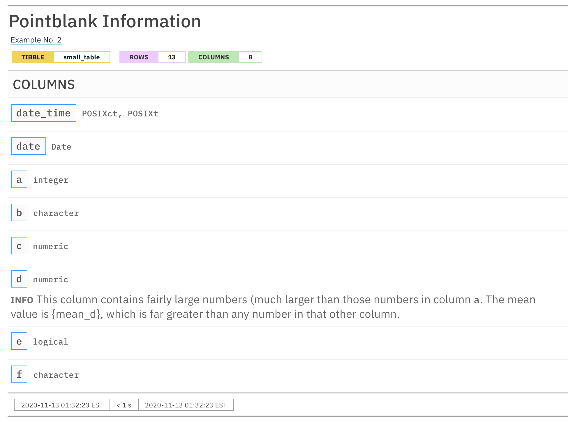

Hmm. There is "... {mean_d} ..." text in the report that should have been replaced with the mean value of column d. What gives? Well, there’s one finalizing step that needs to be done and should always be done to wrap up the Information Management workflow and that is the use of the incorporate() function. Let’s write the whole thing again and finish it off with a call to incorporate().

informant <- 
  create_informant(
    tbl = small_table,
    tbl_name = "small_table",
    label = "Example No. 2"
  ) %>%
  info_snippet(
    snippet_name = "mean_d",
    fn = ~ . %>% .$d %>% mean() %>% round(1)
  ) %>%
    info_columns(
    columns = d,
    info = "This column contains fairly large numbers (much larger than
    those numbers in column `a`. The mean value is {mean_d}, which is
    far greater than any number in that other column."
  ) %>%
  incorporate()

informant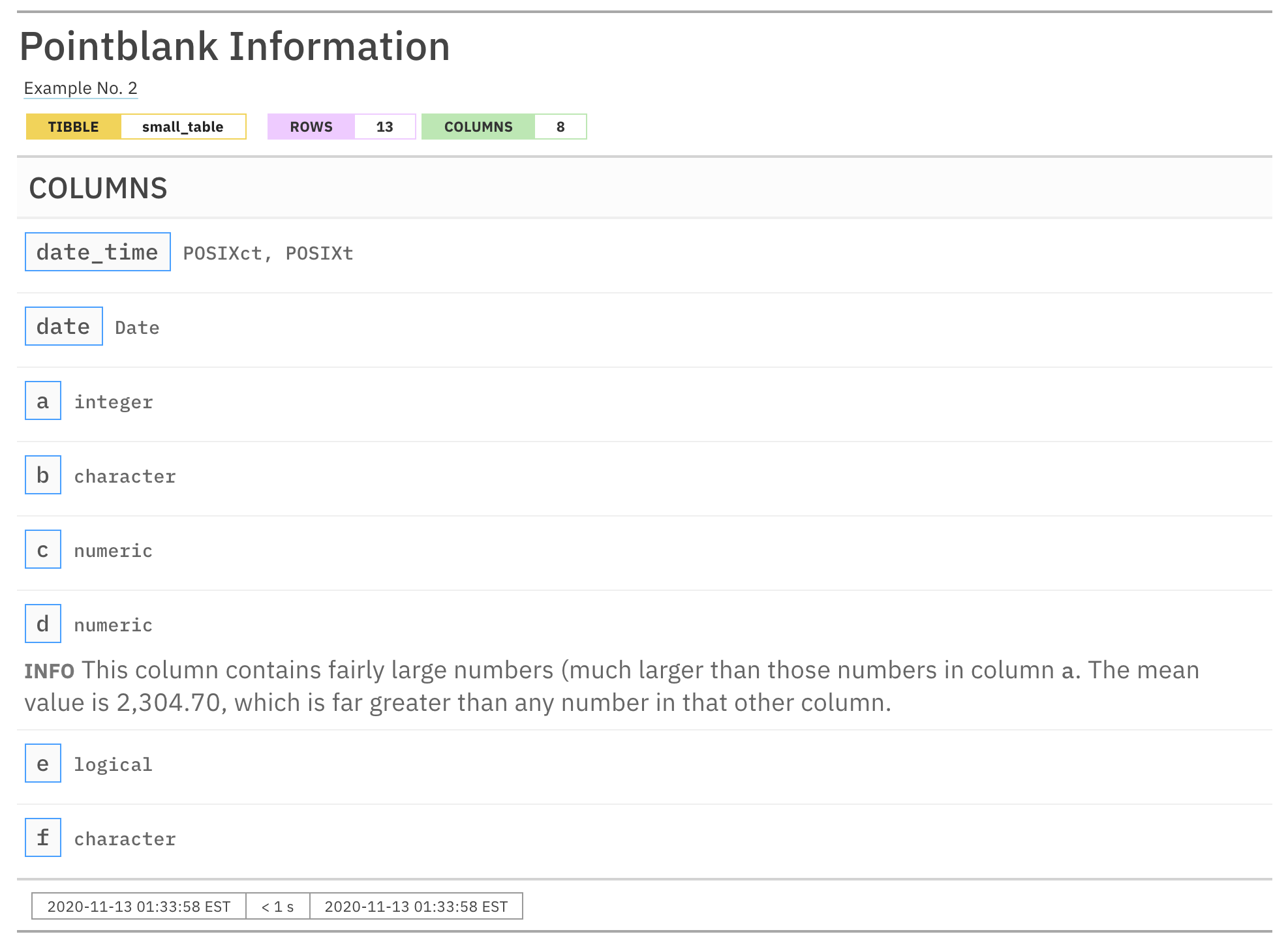

This time, sweet success. The value appears and the overall formatting looks great! This is a very useful thing, so long as we remember to use the incorporate() function to make it happen (more on that in the next section).

Ensuring That Snippets (and Other Table Metadata Element) Are Up-to-Date

Tables can change with time. Whether that data source is a public dataset, an organization’s data table, or a continually-updated Excel file (😱), we should be ready for change. In the previous example, we used the incorporate() function to finalize the report. Without it, our snippet didn’t work. There are two major things that incorporate() does for you in the Information Management workflow.

1. Evaluation of text snippets in all info_snippet() calls, and, insertion of snippets in info text within "{<snippet_name>}".

2. Updating of table row and column counts in the header of the report.

We really are incorporating aspects of the table into the report with incorporate() but might also think of it as regenerating, refreshing, or renewing the table. It gives pointblank license to access the table the same way that interrogate() does in the VALID-I validation workflow. On the first use of incorporate(), all text snippets will be put in their places; subsequent uses of incorporate() will replace the appropriate text as necessary. Every use of incorporate() will update the row and column counts in the header.

Here’s a short demo of the header changing, because it’s pretty instructive. Let’s use our small_table object as target_table. With dim() we can be totally sure of the table dimensions.

target_table <- small_table

dim(target_table)

## [1] 13  8

Let’s allow an informant to access the target_table through the tbl argument but, in this case, the expression is ~ target_table (it simply gets the table from the global workspace). After using incorporate() and printing the informant_tt object, let’s just examine the header.

informant_tt <- 
  create_informant(
    tbl = ~ target_table,
    tbl_name = "target_table",
    label = "Example No. 3"
  ) %>%
  incorporate()

informant_tt

This is an excerpt of the complete report, showing just the header.

The number of rows and columns reported in the header checks out: 13 rows and 8 columns.

Now, let’s manually enlarge the target_table and print the new row and column counts.

target_table <- 
  dplyr::bind_rows(small_table, small_table) %>%
  dplyr::mutate(g = a + c)

dim(target_table)

## [1] 26  9

We’ve got our informant object, let’s see how incorporate() keeps pace with the change.

informant_tt %>% incorporate()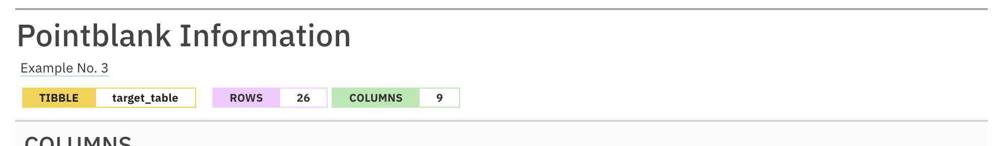

This is an excerpt of the complete report, showing just the header.

Great! Using incorporate() has accurately updated the reporting of row and column counts in the header. And it’s also very much worth noting that the use of tbl = ~ target_table rather than tbl = target_table is important here. Had the latter been used in create_informant(), that table would be bound to the informant in its initial state (with 13 rows and 8 columns) and any updates to the table wouldn’t be reflected in the reporting upon using incorporate(). The table-prep formula used here is meant for re-obtaining the table each and every time the table is needed.

In short, unless you have no uses of info_snippet() and the table isn’t expected to change, it’s recommended to use incorporate() as the final call in this workflow.

Helpful pointblank Functions that Work Exceedingly Well with info_snippet()

There are a few functions available in pointblank that make it much easier to get commonly-used text snippets. All of them begin with the snip_ prefix and they are:

• snip_list(): Gets a list of column categories
• snip_lowest(): Gets the lowest value from a column
• snip_highest(): Gets the highest value from a column

Each of these functions can be used directly as a fn value and we don’t have to specify the table since its assumed that the target table is where we’ll be snipping data from. Let’s have a look at each of these in action.

The snip_list() Function

When describing some aspect of the target table, we may want to extract some values from a column and include them as a piece of info text. We’d want the values to be nicely formatted as a list (with commas) and we’d probably prefer that this be constrained to a certain size (so as to not potentially generate massive amounts of text). This can be efficiently done with snip_list(). Let’s experiment with the combination of snip_list() and info_snippet(), extending the palmerpenguins example from the Intro to Information Management article.

informant_pp <- 
  create_informant(
    tbl = ~ palmerpenguins::penguins,
    tbl_name = "penguins",
    label = "The `penguins` dataset from the **palmerpenguins** 📦."
  ) %>% 
  info_columns(
    columns = species,
    `ℹ️` = "A factor denoting penguin species ({species_snippet})."
  ) %>%
  info_columns(
    columns = island,
    `ℹ️` = "A factor denoting island in Palmer Archipelago, Antarctica
    ({island_snippet})."
  ) %>%
  info_snippet(
    snippet_name = "species_snippet",
    fn = snip_list(column = "species")
  ) %>%
  info_snippet(
    snippet_name = "island_snippet",
    fn = snip_list(column = "island")
  ) %>%
  incorporate()

informant_pp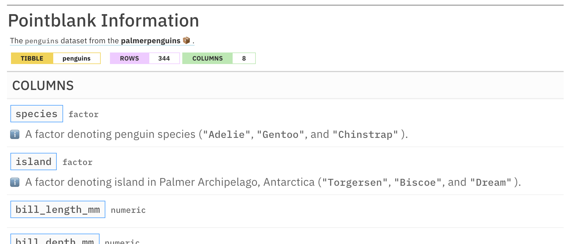

This is an excerpt of the complete report, showing just the header and part of the COLUMNS section.

This seemed to work out quite well. No need for determining what these strings are and then hardcoding them to the info text, snip_list() did all the work here.

This also works for numeric values. Let’s use snip_list() to provide a text snippet based on values in the year column (which is an integer column):

informant_pp <-
  informant_pp %>%
  info_columns(
    columns = year,
    `ℹ️` = "The study year ({year_snippet})."
  ) %>%
  info_snippet(
    snippet_name = "year_snippet",
    fn = snip_list(column = "year")
  ) %>%
  incorporate()

informant_pp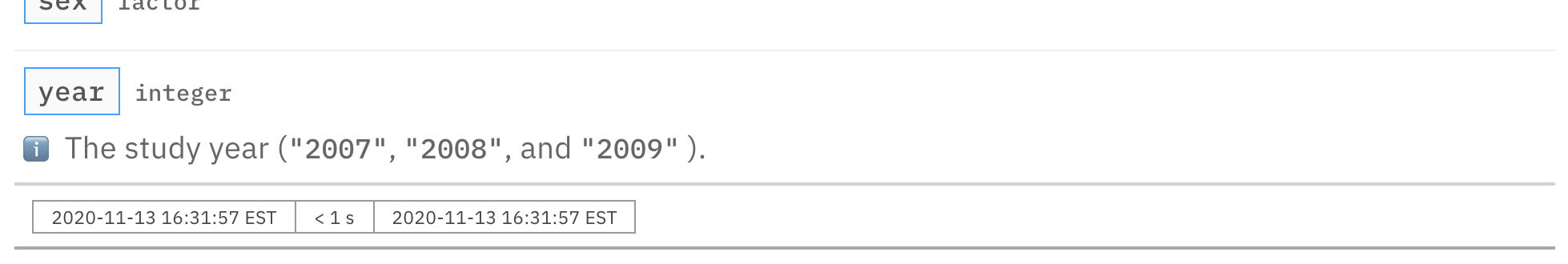

This is an excerpt of the complete report, showing just the bottom of the COLUMNS section and the footer.

Again, no issues with the formatting and display of values. We got the info text "The study year ("2007", "2008", and "2009" )." for our efforts here and it saved us from having to determine this, plus, should the data be updated with new year values, that will be reflected in this info text upon using incorporate(). Refreshed info text really provides huge benefits, especially when the data changes a lot (e.g., database tables).

The snip_lowest() and snip_highest() Functions

We can get the lowest and highest values from a column and inject those formatted values into some info_text. Let’s do that for some of the measured values in the penguins dataset with snip_lowest() and snip_highest().

informant_pp <-
  informant_pp %>%
  info_columns(
    columns = bill_length_mm,
    `ℹ️` = "A number denoting bill length"
  ) %>%
  info_columns(
    columns = bill_depth_mm,
    `ℹ️` = "A number denoting bill depth (in the range of
    {min_depth} to {max_depth} millimeters)."
  ) %>%
  info_columns(
    columns = flipper_length_mm,
    `ℹ️` = "An integer denoting flipper length"
  ) %>%
  info_columns(
    columns = matches("length"),
    `ℹ️` = "(in units of millimeters)."
  ) %>%
  info_columns(
    columns = flipper_length_mm,
    `ℹ️` = "Largest observed is {largest_flipper_length} mm."
  ) %>%
  info_snippet(
    snippet_name = "min_depth",
    fn = snip_lowest(column = "bill_depth_mm")
  ) %>%
  info_snippet(
    snippet_name = "max_depth",
    fn = snip_highest(column = "bill_depth_mm")
  ) %>%
  info_snippet(
    snippet_name = "largest_flipper_length",
    fn = snip_highest(column = "flipper_length_mm")
  ) %>%
  incorporate()

informant_pp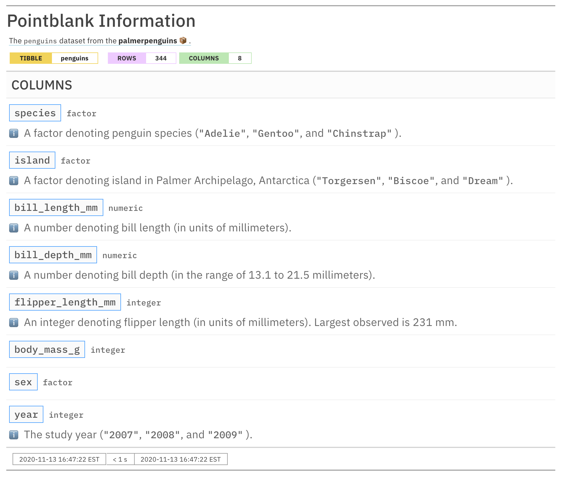

We can see from the report output that we can creatively use the lowest and highest values obtained by snip_lowest() and snip_highest() to specify a range or simply show some maximum value. While the ordering of the info_columns() calls in the example affects the overall layout of the text (through the text appending behavior), the placement of info_snippet() calls does not matter. And, again, we must use incorporate() to update all of the text snippets and render them in their appropriate locations (inside each {<snippet_name>}).

Text Tricks

While your info text can be jazzed up with Markdown, there are a few extra tricks that make authoring the text a bit more pleasurable. Once you know about these text tricks you’ll be able to express information in many more interesting ways.

Links and Dates

If you have links in your text, pointblank will try to identify them and style them nicely. This amounts to using a pleasing, light-blue color and underlines that appear on hover. It doesn’t take much to style links but it does require something. So, Markdown links written as < link url > or [ link text ]( link url ) will both get the transformation treatment.

Sometimes you want dates to stand out from text. Try enclosing a date expressed in the ISO-8601 standard with parentheses, like this: (2004-12-01). What will happen is that date will be set in a monospaced variation of the reporting font, and, it will be underlined in a striking shade of purple.

Here’s how we might use these features while otherwise adding more information to the palmerpenguins reporting:

informant_pp <-
  informant_pp %>%
  info_tabular(
    `R dataset` = "The goal of `palmerpenguins` is to provide a great dataset
    for data exploration & visualization, as an alternative to `iris`. The
    latest CRAN release was published on (2020-07-25).",
    `data collection` = "Data were collected and made available by Dr. Kristen
    Gorman and the [Palmer Station, Antarctica LTER](https://pal.lternet.edu),
    a member of the [Long Term Ecological Research Network](https://lternet.edu).",
    citation = "Horst AM, Hill AP, Gorman KB (2020). palmerpenguins: Palmer 
    Archipelago (Antarctica) penguin data. R package version 0.1.0.
    <https://allisonhorst.github.io/palmerpenguins/>. 
    doi: 10.5281/zenodo.3960218."
  ) %>%
  incorporate()

informant_pp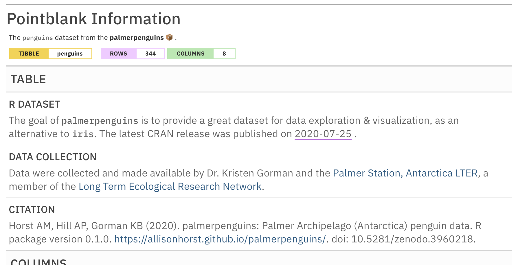

This is an excerpt of the complete report, showing just the TABLE section and the header.

Labels

We can take portions of text and present them as labels. These will help you call out important attributes in short form and may eliminate the need for oft-repeated statements. You might apply to labels to signify priority, category, or any other information you find useful. To do this we have two options,

1. Use double parentheses around text to capture it in a rectangular label: ((label text))
2. Use triple parentheses to capture text into a rounded-rectangular label: (((label text)))

informant_pp <-
  informant_pp %>%
  info_columns(
    columns = body_mass_g, 
    `ℹ️` = "An integer denoting body mass."
  ) %>%
  info_columns(
    columns = c(ends_with("mm"), ends_with("g")),
    `ℹ️` = "((measured))"    
  ) %>%
  info_section(
    section_name = "additional notes",
    `data types` = "(((factor))) (((numeric))) (((integer)))"
  ) %>%
  incorporate()

informant_pp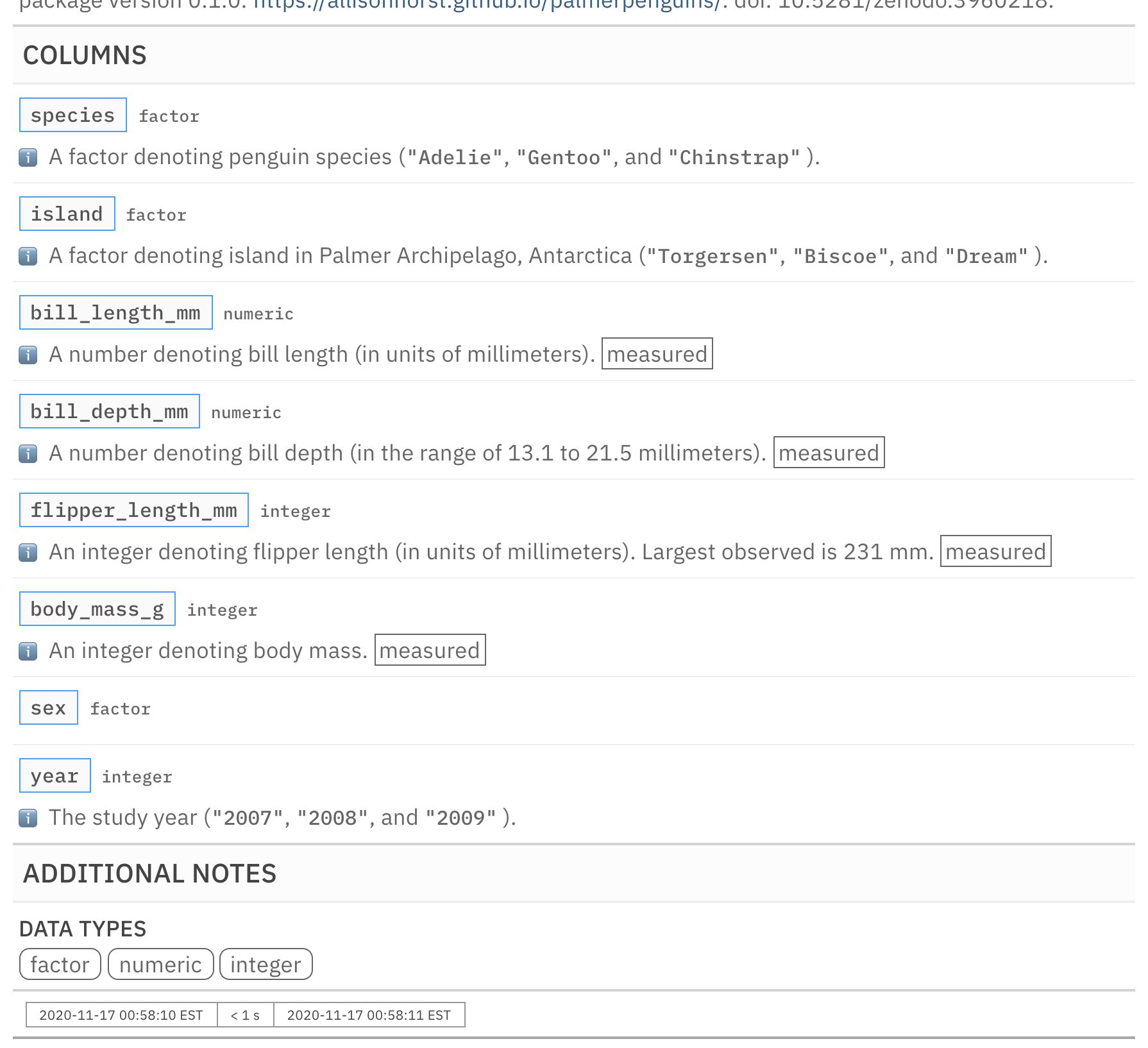

This is an excerpt of the complete report, showing just the COLUMNS and ADDITIONAL NOTES sections.

Get Stylin’

If you want to use CSS styles on spans of info text, it’s possible with the following construction:

[[ info text ]]<< CSS style rules >>

It’s important to ensure that each CSS rule is concluded with a ; character in this syntax. Styling the word factor inside a piece of info text might look like this:

This is a [[factor]]<<color: red; font-weight: 300;>> value.

Where the result looks something like this:

There are many CSS style rules that can be used. Here’s a sample of a few useful ones:

• color: <a color value>; (text color)
• background-color: <a color value>; (the text’s background color)
• text-decoration: (overline | line-through | underline);
• text-transform: (uppercase | lowercase | capitalize);
• letter-spacing: <a +/- length value>;
• word-spacing: <a +/- length value>;
• font-style: (normal | italic | oblique);
• font-weight: (normal | bold | 100-900);
• font-variant: (normal | bold | 100-900);
• border: <a color value> <a length value> (solid | dashed | dotted);

Continuing with our palmerpenguins reporting, we’ll add some more info text and take the opportunity to add CSS style rules using the [[ ]]<< >> syntax.

informant_pp <-
  informant_pp %>%
  info_columns(
    columns = sex, 
    `ℹ️` = "A [[factor]]<<text-decoration: underline;>> 
    denoting penguin sex (female or male)."
  ) %>%
  info_section(
    section_name = "additional notes",
    keywords = "
    [[((penguins))]]<<border-color: platinum; background-color: #F0F8FF;>>
     [[((Antarctica))]]<<border-color: #800080; background-color: #F2F2F2;>>
     [[((measurements))]]<<border-color: #FFB3B3; background-color: #FFFEF4;>>
    "
  ) %>%
  incorporate()

informant_pp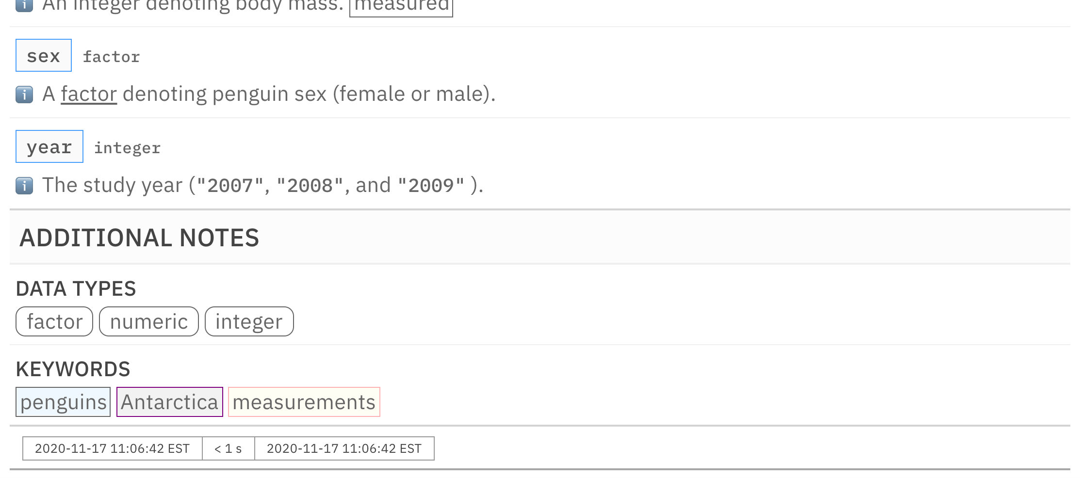

This is an excerpt of the complete report, showing just the bottom of the COLUMNS section, the ADDITIONAL NOTES section, and the footer.

With the above info_columns() and info_section() function calls, we are able to style a single word (with an underline) and even style labels (changing the border and background colors). The syntax here is somewhat forgiving, allowing you to put line breaks between ]] and << and between style rules so that lines of markup don’t have to be overly long.

So, what do you think of all these text tricks? You got to admit they can spice up the proceedings. More of them will inevitably be added as development on pointblank proceeds. But that’s it for now. Don’t you think you’ve had enough?